Disclaimer: This post has been translated to English using a machine translation model. Please, let me know if you find any mistakes.
1. Summary
Let's take a look at a brief introduction to the data manipulation and analysis library Pandas. With it, we can handle and process tabular data, which will help us operate with the data and extract valuable information.
![]()
2. What is Pandas?
Pandas is a **Python** library designed to make working with *relational* or *labeled* data easy and intuitive
Pandas is designed for many different types of data:
- Tabular data with heterogeneous column types, such as in an SQL table or an Excel spreadsheet
- Time series data, ordered and unordered (not necessarily of fixed frequency).
- Arbitrary matrix data (homogeneous or heterogeneous) with row and column labels
- Any other form of observational/statistical datasets. Data does not need to be labeled at all in order to place it into a Pandas data structure.
The two main data structures of Pandas are Series (one-dimensional) and DataFrames (two-dimensional). Pandas is built on top of NumPy and is designed to integrate well within a scientific computing environment with many other third-party libraries.
For data scientists, working with data is generally divided into several stages: collecting and cleaning data, analyzing/modeling it, and then organizing the analysis results in a suitable format for plotting or displaying them in tabular form. pandas is the ideal tool for all these tasks.
Another feature is that pandas is fast, many of the low-level algorithms have been built in C.
2.1. Pandas as pd
Generally when importing pandas, it is usually imported with the alias pd
InputPythonimport pandas as pdprint(pd.__version__)Copied
1.0.1
3. Data Structures in Pandas
In Pandas there are two types of data structures: Series and DataFrames
3.1. Series
The Serie data type is a one-dimensional labeled array capable of holding any data type (integers, strings, floating-point numbers, Python objects, etc.). It is divided into indices.
To create a Series data type, the most common way is
series = pd.Series(data, index=index)Where data can be:
- A dictionary* A list or tuple
- A
ndarrayfrom Numpy - A scalar value
As one of the data types can be a ndarray from NumPy, we import NumPy to be able to use it
InputPythonimport numpy as npCopied
3.1.1. Series from a dictionary
InputPythondiccionario = {"b": 1, "a": 0, "c": 2}serie = pd.Series(diccionario)serieCopied
b 1a 0c 2dtype: int64
If an index is passed, the values corresponding to the index labels will be extracted. If they do not exist, they are created as NaN (not a number)
InputPythondiccionario = {"b": 1, "a": 0, "c": 2}serie = pd.Series(diccionario, index=["b", "c", "d", "a"])serieCopied
b 1.0c 2.0d NaNa 0.0dtype: float64
3.1.2. Series from a list or tuple
If the data comes from a list or tuple and no index is passed, one will be created with values [0, ..., len(data)-1]
InputPythonserie = pd.Series([1, 2, 3, 4])serieCopied
0 11 22 33 4dtype: int64
If an index is passed, it must have the same length as the data
InputPythonserie = pd.Series([1, 2, 3, 4], index=["a", "b", "c", "d"])serieCopied
a 1b 2c 3d 4dtype: int64
3.1.3. Series from an ndarray
If the data comes from an ndarray and no index is passed, one will be created with values [0, ..., len(data)-1]
InputPythonserie = pd.Series(np.random.randn(5))serieCopied
0 1.2678651 -0.8778572 -0.1385563 -0.1329874 -0.827295dtype: float64
If an index is passed, it must have the same length as the data
InputPythonserie = pd.Series(np.random.randn(5), index=["a", "b", "c", "d", "e"])serieCopied
a -1.091828b -0.584243c 0.220398d 1.248923e 1.652351dtype: float64
3.1.4. Series from a scalar
If the series is created from a scalar, it will be created with a single item
InputPythonserie = pd.Series(5.0)serieCopied
0 5.0dtype: float64
If you want to create more items in the series, you need to pass the index with the number of items you want, so all the items will have the value of the scalar
InputPythonserie = pd.Series(5.0, index=["a", "b", "c", "d", "e"])serieCopied
a 5.0b 5.0c 5.0d 5.0e 5.0dtype: float64
3.1.5. Operations with Series
Just like with Numpy, we can perform operations on all elements of a series without having to iterate through each one of them.
InputPythonserie = pd.Series(5.0, index=["a", "b", "c", "d", "e"])print(f"serie: {serie}")print(f" serie + serie = {serie + serie}")Copied
serie:a 5.0b 5.0c 5.0d 5.0e 5.0dtype: float64serie + serie =a 10.0b 10.0c 10.0d 10.0e 10.0dtype: float64
InputPythonserie = pd.Series(5.0, index=["a", "b", "c", "d", "e"])print(f"serie: {serie}")print(f" exp(serie) = {np.exp(serie)}")Copied
serie:a 5.0b 5.0c 5.0d 5.0e 5.0dtype: float64exp(serie) =a 148.413159b 148.413159c 148.413159d 148.413159e 148.413159dtype: float64
A difference between Series and ndarrays is that operations between Series automatically align the data according to their labels. Therefore, calculations can be written without considering whether the involved Series have the same labels. If a label is not found in one Series or the other, the result will be marked as missing (NaN).
InputPythonserie = pd.Series(5.0, index=["a", "b", "c", "d", "e"])print(f"serie: {serie}")print(f" serie[1:] + serie[:-1] = {serie[1:] + serie[:-1]}")Copied
serie:a 5.0b 5.0c 5.0d 5.0e 5.0dtype: float64serie[1:] + serie[:-1] =a NaNb 10.0c 10.0d 10.0e NaNdtype: float64
3.1.6. Attribute name of the Series
One of the attributes of Series is name, which corresponds to the name they will have when added to a DataFrame. Conversely, when a series is obtained from a DataFrame, this series will have the same name it had in the DataFrame.
InputPythonserie = pd.Series(np.random.randn(5), name="aleatorio")serieCopied
0 -0.1910091 -0.7931512 -0.9077473 -1.4405084 -0.676419Name: aleatorio, dtype: float64
The name of a series can be changed using the rename() method.
InputPythonserie = serie.rename("random")serieCopied
0 -0.1910091 -0.7931512 -0.9077473 -1.4405084 -0.676419Name: random, dtype: float64
3.2. DataFrames
A DataFrame is a labeled and two-dimensional data structure, with potentially different types of columns, meaning that one column can contain integer data, another column string data, etc. You can think of it as a spreadsheet or an SQL table, or a dictionary of Series objects.
It is the most used pandas object. Just like Series, DataFrames accept many different types of input:
Along with the data, you can optionally pass index arguments (row labels) and columns (column labels). If you pass an index and/or columns, you are guaranteeing the index and/or columns of the resulting DataFrame. Therefore, a dictionary of Series plus a specific index will discard all data that does not match the passed index.
If axis labels are not provided, they will be constructed from the input data based on common sense rules.
3.2.1. DataFrames from a Dictionary of Series
If a dictionary of Series is passed, the DataFrame will be created with as many columns as Series the dictionary has.
InputPythondiccionario = {"uno": pd.Series([1.0, 2.0, 3.0]),"dos": pd.Series([4.0, 5.0, 6.0, 7.0])}dataframe = pd.DataFrame(diccionario)dataframeCopied
uno dos0 1.0 4.01 2.0 5.02 3.0 6.03 NaN 7.0
If each of the Series has defined indices, the resulting DataFrame will be the union of these indices.
InputPythondiccionario = {"uno": pd.Series([1.0, 2.0, 3.0], index=["a", "b", "c"]),"dos": pd.Series([4.0, 5.0, 6.0, 7.0], index=["a", "b", "c", "d"])}dataframe = pd.DataFrame(diccionario)dataframeCopied
uno dosa 1.0 4.0b 2.0 5.0c 3.0 6.0d NaN 7.0
InputPythondataframe = pd.DataFrame(diccionario, index=["d", "b", "a"])dataframeCopied
uno dosd NaN 7.0b 2.0 5.0a 1.0 4.0
If the columns are passed, they will appear in the passed order
InputPythondataframe = pd.DataFrame(diccionario, columns=["dos", "tres"])dataframeCopied
dos tresa 4.0 NaNb 5.0 NaNc 6.0 NaNd 7.0 NaN
3.2.2. DataFrames from a dictionary of ndarrays or lists
All ndarrays or lists must have the same length. If an index is passed, it must also have the same length as the ndarrays or lists.
InputPythondiccionario = {"uno": [1.0, 2.0, 3.0, 4.0],"dos": [4.0, 3.0, 2.0, 1.0]}dataframe = pd.DataFrame(diccionario)dataframeCopied
uno dos0 1.0 4.01 2.0 3.02 3.0 2.03 4.0 1.0
3.2.3. DataFrames from a matrix
If an index is passed, it must have the same length as the number of rows in the array, and if columns are passed, they must have the same length as the columns in the array.
InputPythonmatriz = np.array([[1, 3], [2, 2], [3, 1]])dataframe = pd.DataFrame(matriz, index=["a", "b", "c"], columns=["columna1", "columna2"])dataframeCopied
columna1 columna2a 1 3b 2 2c 3 1
3.2.4. DataFrames from a list of dictionaries
InputPythonlista = [{"a": 1, "b": 2}, {"a": 5, "b": 10, "c": 20}]dataframe = pd.DataFrame(lista)dataframeCopied
a b c0 1 2 NaN1 5 10 20.0
3.2.5. DataFrames from a dictionary of tuples
InputPythondiccionario = {("a", "b"): {("A", "B"): 1, ("A", "C"): 2},("a", "a"): {("A", "C"): 3, ("A", "B"): 4},("a", "c"): {("A", "B"): 5, ("A", "C"): 6},("b", "a"): {("A", "C"): 7, ("A", "B"): 8},("b", "b"): {("A", "D"): 9, ("A", "B"): 10},}dataframe = pd.DataFrame(diccionario)dataframeCopied
a bb a c a bA B 1.0 4.0 5.0 8.0 10.0C 2.0 3.0 6.0 7.0 NaND NaN NaN NaN NaN 9.0
3.2.6. DataFrames from a Series
The result will be a DataFrame with the same index as the input Series, and with a column whose name is the original name of the Series (only if another column name is not provided).
InputPythondiccionario = {"b": 1, "a": 0, "c": 2}serie = pd.Series(diccionario)dataframe = pd.DataFrame(serie)dataframeCopied
0b 1a 0c 2
4. Exploration of a DataFrame
When a DataFrame is very large, it cannot be fully represented.
InputPythoncalifornia_housing_train = pd.read_csv("https://raw.githubusercontent.com/maximofn/portafolio/main/posts/california_housing_train.csv")california_housing_trainCopied
longitude latitude housing_median_age total_rooms total_bedrooms \0 -114.31 34.19 15.0 5612.0 1283.01 -114.47 34.40 19.0 7650.0 1901.02 -114.56 33.69 17.0 720.0 174.03 -114.57 33.64 14.0 1501.0 337.04 -114.57 33.57 20.0 1454.0 326.0... ... ... ... ... ...16995 -124.26 40.58 52.0 2217.0 394.016996 -124.27 40.69 36.0 2349.0 528.016997 -124.30 41.84 17.0 2677.0 531.016998 -124.30 41.80 19.0 2672.0 552.016999 -124.35 40.54 52.0 1820.0 300.0population households median_income median_house_value0 1015.0 472.0 1.4936 66900.01 1129.0 463.0 1.8200 80100.02 333.0 117.0 1.6509 85700.03 515.0 226.0 3.1917 73400.04 624.0 262.0 1.9250 65500.0... ... ... ... ...16995 907.0 369.0 2.3571 111400.016996 1194.0 465.0 2.5179 79000.016997 1244.0 456.0 3.0313 103600.016998 1298.0 478.0 1.9797 85800.016999 806.0 270.0 3.0147 94600.0[17000 rows x 9 columns]
So it's very useful to have methods for exploring it and getting information quickly.
4.1. DataFrame Header
To view the first rows and get an idea of what the DataFrame looks like, there is the head() method, which by default displays the first 5 rows of the DataFrame. If you want to see a different number of rows, specify it using the n attribute.
InputPythoncalifornia_housing_train.head(n=10)Copied
longitude latitude housing_median_age total_rooms total_bedrooms \0 -114.31 34.19 15.0 5612.0 1283.01 -114.47 34.40 19.0 7650.0 1901.02 -114.56 33.69 17.0 720.0 174.03 -114.57 33.64 14.0 1501.0 337.04 -114.57 33.57 20.0 1454.0 326.05 -114.58 33.63 29.0 1387.0 236.06 -114.58 33.61 25.0 2907.0 680.07 -114.59 34.83 41.0 812.0 168.08 -114.59 33.61 34.0 4789.0 1175.09 -114.60 34.83 46.0 1497.0 309.0population households median_income median_house_value0 1015.0 472.0 1.4936 66900.01 1129.0 463.0 1.8200 80100.02 333.0 117.0 1.6509 85700.03 515.0 226.0 3.1917 73400.04 624.0 262.0 1.9250 65500.05 671.0 239.0 3.3438 74000.06 1841.0 633.0 2.6768 82400.07 375.0 158.0 1.7083 48500.08 3134.0 1056.0 2.1782 58400.09 787.0 271.0 2.1908 48100.0
4.2. Tail of the DataFrame
If you want to see the last rows, you can use the tail() method. By using the n parameter, you can choose how many rows to display.
InputPythoncalifornia_housing_train.tail()Copied
longitude latitude housing_median_age total_rooms total_bedrooms \16995 -124.26 40.58 52.0 2217.0 394.016996 -124.27 40.69 36.0 2349.0 528.016997 -124.30 41.84 17.0 2677.0 531.016998 -124.30 41.80 19.0 2672.0 552.016999 -124.35 40.54 52.0 1820.0 300.0population households median_income median_house_value16995 907.0 369.0 2.3571 111400.016996 1194.0 465.0 2.5179 79000.016997 1244.0 456.0 3.0313 103600.016998 1298.0 478.0 1.9797 85800.016999 806.0 270.0 3.0147 94600.0
4.3. DataFrame Information
Another very useful method is info() which gives us information about the DataFrame
InputPythoncalifornia_housing_train.info()Copied
<class 'pandas.core.frame.DataFrame'>RangeIndex: 17000 entries, 0 to 16999Data columns (total 9 columns):# Column Non-Null Count Dtype--- ------ -------------- -----0 longitude 17000 non-null float641 latitude 17000 non-null float642 housing_median_age 17000 non-null float643 total_rooms 17000 non-null float644 total_bedrooms 17000 non-null float645 population 17000 non-null float646 households 17000 non-null float647 median_income 17000 non-null float648 median_house_value 17000 non-null float64dtypes: float64(9)memory usage: 1.2 MB
4.4. Rows and Columns of DataFrame
The indices and columns of a DataFrame can be obtained using the index and columns methods.
InputPythondiccionario = {"uno": pd.Series([1.0, 2.0, 3.0], index=["a", "b", "c"]),"dos": pd.Series([4.0, 5.0, 6.0, 7.0], index=["a", "b", "c", "d"])}dataframe = pd.DataFrame(diccionario)indices = dataframe.indexcolumnas = dataframe.columnsprint(f"El DataFrame tiene los índices {indices} ")print(f"El DataFrame tiene las columnas {columnas}")Copied
El DataFrame tiene los índicesIndex(['a', 'b', 'c', 'd'], dtype='object')El DataFrame tiene las columnasIndex(['uno', 'dos'], dtype='object')
4.5. Description of the DataFrame
The describe() method displays a quick statistical summary of the data in the DataFrame
InputPythoncalifornia_housing_train = pd.read_csv("https://raw.githubusercontent.com/maximofn/portafolio/main/posts/california_housing_train.csv")california_housing_train.describe()Copied
longitude latitude housing_median_age total_rooms \count 17000.000000 17000.000000 17000.000000 17000.000000mean -119.562108 35.625225 28.589353 2643.664412std 2.005166 2.137340 12.586937 2179.947071min -124.350000 32.540000 1.000000 2.00000025% -121.790000 33.930000 18.000000 1462.00000050% -118.490000 34.250000 29.000000 2127.00000075% -118.000000 37.720000 37.000000 3151.250000max -114.310000 41.950000 52.000000 37937.000000total_bedrooms population households median_income \count 17000.000000 17000.000000 17000.000000 17000.000000mean 539.410824 1429.573941 501.221941 3.883578std 421.499452 1147.852959 384.520841 1.908157min 1.000000 3.000000 1.000000 0.49990025% 297.000000 790.000000 282.000000 2.56637550% 434.000000 1167.000000 409.000000 3.54460075% 648.250000 1721.000000 605.250000 4.767000max 6445.000000 35682.000000 6082.000000 15.000100median_house_valuecount 17000.000000mean 207300.912353std 115983.764387min 14999.00000025% 119400.00000050% 180400.00000075% 265000.000000max 500001.000000
4.6. Sorting the DataFrame
Rows of a DataFrame can be alphabetically sorted using the sort_index() method.
InputPythoncalifornia_housing_train = pd.read_csv("https://raw.githubusercontent.com/maximofn/portafolio/main/posts/california_housing_train.csv")california_housing_train.sort_index().head()Copied
longitude latitude housing_median_age total_rooms total_bedrooms \0 -114.31 34.19 15.0 5612.0 1283.01 -114.47 34.40 19.0 7650.0 1901.02 -114.56 33.69 17.0 720.0 174.03 -114.57 33.64 14.0 1501.0 337.04 -114.57 33.57 20.0 1454.0 326.0population households median_income median_house_value0 1015.0 472.0 1.4936 66900.01 1129.0 463.0 1.8200 80100.02 333.0 117.0 1.6509 85700.03 515.0 226.0 3.1917 73400.04 624.0 262.0 1.9250 65500.0
Since the rows were already sorted in this case, we set ascending=False to reverse the order.
InputPythoncalifornia_housing_train.sort_index(ascending=False).head()Copied
longitude latitude housing_median_age total_rooms total_bedrooms \16999 -124.35 40.54 52.0 1820.0 300.016998 -124.30 41.80 19.0 2672.0 552.016997 -124.30 41.84 17.0 2677.0 531.016996 -124.27 40.69 36.0 2349.0 528.016995 -124.26 40.58 52.0 2217.0 394.0population households median_income median_house_value16999 806.0 270.0 3.0147 94600.016998 1298.0 478.0 1.9797 85800.016997 1244.0 456.0 3.0313 103600.016996 1194.0 465.0 2.5179 79000.016995 907.0 369.0 2.3571 111400.0
If you want to sort the columns, you need to set axis=1 since the default is 0.
InputPythoncalifornia_housing_train.sort_index(axis=1).head()Copied
households housing_median_age latitude longitude median_house_value \0 472.0 15.0 34.19 -114.31 66900.01 463.0 19.0 34.40 -114.47 80100.02 117.0 17.0 33.69 -114.56 85700.03 226.0 14.0 33.64 -114.57 73400.04 262.0 20.0 33.57 -114.57 65500.0median_income population total_bedrooms total_rooms0 1.4936 1015.0 1283.0 5612.01 1.8200 1129.0 1901.0 7650.02 1.6509 333.0 174.0 720.03 3.1917 515.0 337.0 1501.04 1.9250 624.0 326.0 1454.0
If we want to sort the DataFrame by a specific column, we need to use the sort_values() method and specify the label of the column to sort by.
InputPythoncalifornia_housing_train.sort_values('median_house_value')Copied
longitude latitude housing_median_age total_rooms total_bedrooms \568 -117.02 36.40 19.0 619.0 239.016643 -122.74 39.71 16.0 255.0 73.016801 -123.17 40.31 36.0 98.0 28.03226 -117.86 34.24 52.0 803.0 267.07182 -118.33 34.15 39.0 493.0 168.0... ... ... ... ... ...15834 -122.42 37.81 52.0 1314.0 317.07927 -118.40 33.87 38.0 2398.0 431.03546 -117.90 33.63 28.0 2370.0 352.07924 -118.40 33.88 35.0 1060.0 191.014011 -122.04 37.26 24.0 4973.0 709.0population households median_income median_house_value568 490.0 164.0 2.1000 14999.016643 85.0 38.0 1.6607 14999.016801 18.0 8.0 0.5360 14999.03226 628.0 225.0 4.1932 14999.07182 259.0 138.0 2.3667 17500.0... ... ... ... ...15834 473.0 250.0 4.3472 500001.07927 911.0 392.0 5.2319 500001.03546 832.0 347.0 7.1148 500001.07924 444.0 196.0 8.0015 500001.014011 1692.0 696.0 7.8627 500001.0[17000 rows x 9 columns]
4.7. DataFrame Statistics
Statistics can be obtained from the DataFrame, such as the mean, mode, and standard deviation.
InputPythoncalifornia_housing_train = pd.read_csv("https://raw.githubusercontent.com/maximofn/portafolio/main/posts/california_housing_train.csv")print(f"media: {california_housing_train.mean()}")print(f" desviación estandar: {california_housing_train.std()}")Copied
media:longitude -119.562108latitude 35.625225housing_median_age 28.589353total_rooms 2643.664412total_bedrooms 539.410824population 1429.573941households 501.221941median_income 3.883578median_house_value 207300.912353dtype: float64desviación estandar:longitude 2.005166latitude 2.137340housing_median_age 12.586937total_rooms 2179.947071total_bedrooms 421.499452population 1147.852959households 384.520841median_income 1.908157median_house_value 115983.764387dtype: float64
If you want to get statistics about the rows instead of the columns, you need to specify it using axis=1
InputPythoncalifornia_housing_train = pd.read_csv("https://raw.githubusercontent.com/maximofn/portafolio/main/posts/california_housing_train.csv")print(f"media: {california_housing_train.mean(axis=1)}")print(f" desviación estandar: {california_housing_train.std(axis=1)}")Copied
media:0 8357.5970671 10131.5277782 9664.6423223 8435.0290784 7567.436111...16995 12806.40856716996 9276.77087816997 12049.50792216998 10082.05330016999 10863.022744Length: 17000, dtype: float64desviación estandar:0 22026.6124451 26352.9392722 28514.3165883 24366.7547474 21730.014569...16995 36979.67689916996 26158.00677116997 34342.87679216998 28408.15232916999 31407.119788Length: 17000, dtype: float64
Another useful thing that can be obtained from DataFrames is, for example, the number of times each item in a column repeats.
InputPythoncalifornia_housing_train["total_rooms"].value_counts()Copied
1582.0 161527.0 151717.0 141471.0 141703.0 14..157.0 12760.0 1458.0 110239.0 14068.0 1Name: total_rooms, Length: 5533, dtype: int64
For example, we can see that there are a total of 16 houses with 1582 rooms.
4.8. Used Memory
We can see the memory used by the DataFrame
InputPythoncalifornia_housing_train.memory_usage(deep=True)Copied
Index 128longitude 136000latitude 136000housing_median_age 136000total_rooms 136000total_bedrooms 136000population 136000households 136000median_income 136000median_house_value 136000dtype: int64
5. Addition of Data
5.1. Addition of Columns
Columns can be easily added as operations of other columns
InputPythondiccionario = {"uno": pd.Series([1.0, 2.0, 3.0]),"dos": pd.Series([4.0, 5.0, 6.0, 7.0])}dataframe = pd.DataFrame(diccionario)dataframe["tres"] = dataframe["uno"] + dataframe["dos"]dataframe["flag"] = dataframe["tres"] > 7.0dataframeCopied
uno dos tres flag0 1.0 4.0 5.0 False1 2.0 5.0 7.0 False2 3.0 6.0 9.0 True3 NaN 7.0 NaN False
Columns can also be added indicating what value all their items will have
InputPythondataframe["constante"] = 8.0dataframeCopied
uno dos tres flag constante0 1.0 4.0 5.0 False 8.01 2.0 5.0 7.0 False 8.02 3.0 6.0 9.0 True 8.03 NaN 7.0 NaN False 8.0
If a Series is added that does not have the same number of indices as the DataFrame, it will be adjusted to match the number of indices of the DataFrame.
InputPythondataframe["Menos indices"] = dataframe["uno"][:2]dataframeCopied
uno dos tres flag constante Menos indices0 1.0 4.0 5.0 False 8.0 1.01 2.0 5.0 7.0 False 8.0 2.02 3.0 6.0 9.0 True 8.0 NaN3 NaN 7.0 NaN False 8.0 NaN
With the previous methods, the column was added at the end, but if you want to add the column in a specific position, you can use the insert() method.
For example, if you want to add a column at position 3 (keeping in mind that indexing starts from position 0), with the name of the column being *inserted column* and its value being double that of the column *three*, it would be done as follows:
InputPythondataframe.insert(loc=3, column="columna insertada", value=dataframe["tres"]*2)dataframeCopied
uno dos tres columna insertada flag constante Menos indices0 1.0 4.0 5.0 10.0 False 8.0 1.01 2.0 5.0 7.0 14.0 False 8.0 2.02 3.0 6.0 9.0 18.0 True 8.0 NaN3 NaN 7.0 NaN NaN False 8.0 NaN
If you want to add more than one column per command, you can use the assign() method.
InputPythondataframe = dataframe.assign(columna_asignada1 = dataframe["uno"] * dataframe["tres"],columna_asignada2 = dataframe["dos"] * dataframe["tres"],)dataframeCopied
uno dos tres ... Menos indices columna_asignada1 columna_asignada20 1.0 4.0 5.0 ... 1.0 5.0 20.01 2.0 5.0 7.0 ... 2.0 14.0 35.02 3.0 6.0 9.0 ... NaN 27.0 54.03 NaN 7.0 NaN ... NaN NaN NaN[4 rows x 9 columns]
5.2. Addition of Rows
InputPythondiccionario = {"uno": pd.Series([1.0, 2.0, 3.0]),"dos": pd.Series([4.0, 5.0, 6.0, 7.0])}dataframe = pd.DataFrame(diccionario)dataframe.head()Copied
uno dos0 1.0 4.01 2.0 5.02 3.0 6.03 NaN 7.0
We can add a row at the end using the concat method (which we will cover in more detail later)
InputPythondiccionario = {"uno": [10.0],"dos": [20.0]}dataframe = pd.concat([dataframe, pd.DataFrame(diccionario)])dataframeCopied
uno dos0 1.0 4.01 2.0 5.02 3.0 6.03 NaN 7.00 10.0 20.0
We see that the column has been added at the end, but it has index zero, so we reorder the indices using the method reset_index(drop=True)
InputPythondataframe = dataframe.reset_index(drop=True)dataframeCopied
index uno dos0 0 1.0 4.01 1 2.0 5.02 2 3.0 6.03 3 NaN 7.04 0 10.0 20.0
6. Data Deletion
6.1. Column Deletion
A specific column can be deleted using the pop() method.
InputPythondataframe.pop("constante")dataframeCopied
uno dos tres ... Menos indices columna_asignada1 columna_asignada20 1.0 4.0 5.0 ... 1.0 5.0 20.01 2.0 5.0 7.0 ... 2.0 14.0 35.02 3.0 6.0 9.0 ... NaN 27.0 54.03 NaN 7.0 NaN ... NaN NaN NaN[4 rows x 8 columns]
Or using del
InputPythondel dataframe["flag"]dataframeCopied
uno dos tres ... Menos indices columna_asignada1 columna_asignada20 1.0 4.0 5.0 ... 1.0 5.0 20.01 2.0 5.0 7.0 ... 2.0 14.0 35.02 3.0 6.0 9.0 ... NaN 27.0 54.03 NaN 7.0 NaN ... NaN NaN NaN[4 rows x 7 columns]
6.1. Row Deletion
InputPythondiccionario = {"uno": pd.Series([1.0, 2.0, 3.0, 4.0, 5.0, 6.0, 7.0, 8.0, 9.0, 10.0]),"dos": pd.Series([11.0, 12.0, 13.0, 14.0, 15.0, 16.0, 17.0, 18.0, 19.0, 20.0]),"tres": pd.Series([21.0, 22.0, 23.0, 24.0, 25.0, 26.0, 27.0, 28.0, 29.0, 30.0])}dataframe = pd.DataFrame(diccionario)dataframe.head()Copied
uno dos tres0 1.0 11.0 21.01 2.0 12.0 22.02 3.0 13.0 23.03 4.0 14.0 24.04 5.0 15.0 25.0
If we want to delete a row, we can use the drop method, specifying its position. For example, if we want to delete the row at position 1
InputPythondataframe = dataframe.drop(1)dataframeCopied
uno dos tres0 1.0 11.0 21.02 3.0 13.0 23.03 4.0 14.0 24.04 5.0 15.0 25.05 6.0 16.0 26.06 7.0 17.0 27.07 8.0 18.0 28.08 9.0 19.0 29.09 10.0 20.0 30.0
If we want to delete the last row
InputPythondataframe = dataframe.drop(len(dataframe)-1)dataframeCopied
uno dos tres0 1.0 11.0 21.02 3.0 13.0 23.03 4.0 14.0 24.04 5.0 15.0 25.05 6.0 16.0 26.06 7.0 17.0 27.07 8.0 18.0 28.09 10.0 20.0 30.0
If what we want is to delete a range of rows
InputPythondataframe = dataframe.drop(range(2, 5))dataframeCopied
uno dos tres0 1.0 11.0 21.05 6.0 16.0 26.06 7.0 17.0 27.07 8.0 18.0 28.09 10.0 20.0 30.0
If what we want is to remove a specific set of rows
InputPythondataframe = dataframe.drop([5, 7, 9])dataframeCopied
uno dos tres0 1.0 11.0 21.06 7.0 17.0 27.0
Just like when we added rows, we see that some indices have been removed, so we reorder the indices using the method reset_index(drop=True)
InputPythondataframe = dataframe.reset_index(drop=True)dataframeCopied
uno dos tres0 1.0 11.0 21.01 7.0 17.0 27.0
7. Operations on DataFrames
Operations can be performed on DataFrames just as they can with Numpy.
InputPythondiccionario = {"uno": pd.Series([1.0, 2.0, 3.0, 4.0, 5.0, 6.0, 7.0, 8.0, 9.0, 10.0]),"dos": pd.Series([11.0, 12.0, 13.0, 14.0, 15.0, 16.0, 17.0, 18.0, 19.0, 20.0]),"tres": pd.Series([21.0, 22.0, 23.0, 24.0, 25.0, 26.0, 27.0, 28.0, 29.0, 30.0])}dataframe = pd.DataFrame(diccionario)dataframe.head()Copied
uno dos tres0 1.0 11.0 21.01 2.0 12.0 22.02 3.0 13.0 23.03 4.0 14.0 24.04 5.0 15.0 25.0
InputPythondataframe[ ["uno", "dos", "tres"] ] * 2Copied
uno dos tres0 2.0 22.0 42.01 4.0 24.0 44.02 6.0 26.0 46.03 8.0 28.0 48.04 10.0 30.0 50.05 12.0 32.0 52.06 14.0 34.0 54.07 16.0 36.0 56.08 18.0 38.0 58.09 20.0 40.0 60.0
InputPythonnp.exp(dataframe[ ["uno", "dos", "tres"] ])Copied
uno dos tres0 2.718282 5.987414e+04 1.318816e+091 7.389056 1.627548e+05 3.584913e+092 20.085537 4.424134e+05 9.744803e+093 54.598150 1.202604e+06 2.648912e+104 148.413159 3.269017e+06 7.200490e+105 403.428793 8.886111e+06 1.957296e+116 1096.633158 2.415495e+07 5.320482e+117 2980.957987 6.565997e+07 1.446257e+128 8103.083928 1.784823e+08 3.931334e+129 22026.465795 4.851652e+08 1.068647e+13
If more complex operations are desired, the apply() method can be used.
InputPythondataframe = dataframe.apply(lambda x: x.max() - x.min())dataframeCopied
uno 9.0dos 9.0tres 9.0dtype: float64
A lambda function has been applied because it is a simple function, but if we want to apply more complex functions, we can define and apply them.
InputPythondef funcion(x):if x < 10:return np.exp(x) - np.log(5*x) + np.sqrt(x)elif x < 20:return np.sin(x) + np.cos(x) + np.tan(x)else:return np.log(x) + np.log10(x) + np.log2(x)dataframe = dataframe.apply(funcion)dataframeCopied
uno 8102.277265dos 8102.277265tres 8102.277265dtype: float64
Using the apply method on a DataFrame is much faster than looping through each row and performing the operation.
InputPythoncalifornia_housing_train = pd.read_csv("https://raw.githubusercontent.com/maximofn/portafolio/main/posts/california_housing_train.csv")california_housing_train.head()Copied
longitude latitude housing_median_age total_rooms total_bedrooms \0 -114.31 34.19 15.0 5612.0 1283.01 -114.47 34.40 19.0 7650.0 1901.02 -114.56 33.69 17.0 720.0 174.03 -114.57 33.64 14.0 1501.0 337.04 -114.57 33.57 20.0 1454.0 326.0population households median_income median_house_value0 1015.0 472.0 1.4936 66900.01 1129.0 463.0 1.8200 80100.02 333.0 117.0 1.6509 85700.03 515.0 226.0 3.1917 73400.04 624.0 262.0 1.9250 65500.0
Let's calculate the percentage of bedrooms out of the total number of rooms.
InputPythoncalifornia_housing_train["percent_bedrooms"] = None%time california_housing_train["percent_bedrooms"] = california_housing_train.apply(lambda x: x["total_bedrooms"] / x["total_rooms"], axis=1)california_housing_train.head()Copied
CPU times: user 309 ms, sys: 86 µs, total: 309 msWall time: 309 ms
longitude latitude housing_median_age total_rooms total_bedrooms \0 -114.31 34.19 15.0 5612.0 1283.01 -114.47 34.40 19.0 7650.0 1901.02 -114.56 33.69 17.0 720.0 174.03 -114.57 33.64 14.0 1501.0 337.04 -114.57 33.57 20.0 1454.0 326.0population households median_income median_house_value percent_bedrooms0 1015.0 472.0 1.4936 66900.0 0.2286171 1129.0 463.0 1.8200 80100.0 0.2484972 333.0 117.0 1.6509 85700.0 0.2416673 515.0 226.0 3.1917 73400.0 0.2245174 624.0 262.0 1.9250 65500.0 0.224209
InputPythoncalifornia_housing_train["percent_bedrooms"] = None%time for i in range(len(california_housing_train)): california_housing_train["percent_bedrooms"][i] = california_housing_train["total_bedrooms"][i] / california_housing_train["total_rooms"][i]california_housing_train.head()Copied
/home/wallabot/anaconda3/lib/python3.7/site-packages/ipykernel_launcher.py:1: SettingWithCopyWarning:A value is trying to be set on a copy of a slice from a DataFrameSee the caveats in the documentation: https://pandas.pydata.org/pandas-docs/stable/user_guide/indexing.html#returning-a-view-versus-a-copy"""Entry point for launching an IPython kernel.
CPU times: user 1.72 s, sys: 12 ms, total: 1.73 sWall time: 1.72 s
longitude latitude housing_median_age total_rooms total_bedrooms \0 -114.31 34.19 15.0 5612.0 1283.01 -114.47 34.40 19.0 7650.0 1901.02 -114.56 33.69 17.0 720.0 174.03 -114.57 33.64 14.0 1501.0 337.04 -114.57 33.57 20.0 1454.0 326.0population households median_income median_house_value percent_bedrooms0 1015.0 472.0 1.4936 66900.0 0.2286171 1129.0 463.0 1.8200 80100.0 0.2484972 333.0 117.0 1.6509 85700.0 0.2416673 515.0 226.0 3.1917 73400.0 0.2245174 624.0 262.0 1.9250 65500.0 0.224209
The lambda function took about 300 ms, while the for loop took more than 1 second.
8. Transpose
The transpose of a DataFrame can be obtained using the T method.
InputPythondiccionario = {"uno": pd.Series([1.0, 2.0, 3.0], index=["fila a", "fila b", "fila c"]),"dos": pd.Series([4.0, 5.0, 6.0], index=["fila a", "fila b", "fila c"])}dataframe = pd.DataFrame(diccionario)dataframe["tres"] = dataframe["uno"] + dataframe["dos"]dataframe["flag"] = dataframe["tres"] > 7.0dataframe.TCopied
fila a fila b fila cuno 1 2 3dos 4 5 6tres 5 7 9flag False False True
9. Conversion to Numpy
If you want to convert a Series or DataFrame to NumPy, you can use the to_numpy() method or the np.asarray() function.
InputPythondiccionario = {"uno": pd.Series([1.0, 2.0, 3.0], index=["fila a", "fila b", "fila c"]),"dos": pd.Series([4.0, 5.0, 6.0], index=["fila a", "fila b", "fila c"])}dataframe = pd.DataFrame(diccionario)dataframe["tres"] = dataframe["uno"] + dataframe["dos"]dataframe["flag"] = dataframe["tres"] > 7.0dataframeCopied
uno dos tres flagfila a 1.0 4.0 5.0 Falsefila b 2.0 5.0 7.0 Falsefila c 3.0 6.0 9.0 True
InputPythonmatriz_np = dataframe.to_numpy()matriz_npCopied
array([[1.0, 4.0, 5.0, False],[2.0, 5.0, 7.0, False],[3.0, 6.0, 9.0, True]], dtype=object)
InputPythonmatriz_np = np.asarray(dataframe)matriz_npCopied
array([[1.0, 4.0, 5.0, False],[2.0, 5.0, 7.0, False],[3.0, 6.0, 9.0, True]], dtype=object)
This example is not the most appropriate, as it mixes numbers with booleans, and as we explained in the previous post Matrix Calculus with NumPy, all elements of an ndarray must be of the same type.
In this case we are mixing numbers with booleans, so to solve it NumPy converts them all to objects
To solve this, we keep only the numbers and convert them to an ndarray
InputPythonmatriz_np = dataframe[ ["uno", "dos", "tres"] ].to_numpy()matriz_np, matriz_np.dtypeCopied
(array([[1., 4., 5.],[2., 5., 7.],[3., 6., 9.]]), dtype('float64'))
Now it can be seen that an ndarray has been created where all the data are of type float
10. Reading data from external sources
One of the greatest strengths of Pandas is being able to read data from files, so it's not necessary to create a DataFrame with the data you want to process; instead, it can be read from a file.
Just like you can create DataFrames from external files, you can also save DataFrames to files, so you can create your own dataset, configure it the way you want, and save it to a file to use it later.
The following table shows the functions for reading and writing files in different formats.
| Format | File type | Reading function | Writing function |
|---|---|---|---|
| text | CSV | [read_csv](https://pandas.pydata.org/pandas-docs/stable/user_guide/io.html#io-read-csv-table) | [to_csv](https://pandas.pydata.org/pandas-docs/stable/user_guide/io.html#io-store-in-csv) |
| text | Fixed-Width Text File | [read_fwf](https://pandas.pydata.org/pandas-docs/stable/user_guide/io.html#io-fwf-reader) | |
| text | JSON | [read_json](https://pandas.pydata.org/pandas-docs/stable/user_guide/io.html#io-json-reader) | [to_json](https://pandas.pydata.org/pandas-docs/stable/user_guide/io.html#io-json-writer) |
| text | HTML | [read_html](https://pandas.pydata.org/pandas-docs/stable/user_guide/io.html#io-read-html) | [to_html](https://pandas.pydata.org/pandas-docs/stable/user_guide/io.html#io-html) |
| text | Local clipboard | [read_clipboard](https://pandas.pydata.org/pandas-docs/stable/user_guide/io.html#io-clipboard) | [to_clipboard](https://pandas.pydata.org/pandas-docs/stable/user_guide/io.html#io-clipboard) |
| binary | MS Excel | [read_excel](https://pandas.pydata.org/pandas-docs/stable/user_guide/io.html#io-excel-reader) | [to_excel](https://pandas.pydata.org/pandas-docs/stable/user_guide/io.html#io-excel-writer) |
| binary | OpenDocument | [read_excel](https://pandas.pydata.org/pandas-docs/stable/user_guide/io.html#io-ods) | |
| binary | HDF5 Format | [read_hdf](https://pandas.pydata.org/pandas-docs/stable/user_guide/io.html#io-hdf5) | [to_hdf](https://pandas.pydata.org/pandas-docs/stable/user_guide/io.html#io-hdf5) |
| binary | Feather Format | [read_feather](https://pandas.pydata.org/pandas-docs/stable/user_guide/io.html#io-feather) | [to_feather](https://pandas.pydata.org/pandas-docs/stable/user_guide/io.html#io-feather) |
| binary | Parquet Format | [read_parquet](https://pandas.pydata.org/pandas-docs/stable/user_guide/io.html#io-parquet) | [to_parquet](https://pandas.pydata.org/pandas-docs/stable/user_guide/io.html#io-parquet) |
| binary | ORC Format | [read_orc](https://pandas.pydata.org/pandas-docs/stable/user_guide/io.html#io-orc) | |
| binary | Msgpack | [read_msgpack](https://pandas.pydata.org/pandas-docs/stable/user_guide/io.html#io-msgpack) | [to_msgpack](https://pandas.pydata.org/pandas-docs/stable/user_guide/io.html#io-msgpack) |
| binary | Stata | [read_stata](https://pandas.pydata.org/pandas-docs/stable/user_guide/io.html#io-stata-reader) | [to_stata](https://pandas.pydata.org/pandas-docs/stable/user_guide/io.html#io-stata-writer) |
| binary | SAS | [read_sas](https://pandas.pydata.org/pandas-docs/stable/user_guide/io.html#io-sas-reader) | |
| binary | SPSS | [read_spss](https://pandas.pydata.org/pandas-docs/stable/user_guide/io.html#io-spss-reader) | |
| binary | Python Pickle Format | [read_pickle](https://pandas.pydata.org/pandas-docs/stable/user_guide/io.html#io-pickle) | [to_pickle](https://pandas.pydata.org/pandas-docs/stable/user_guide/io.html#io-pickle) |
| SQL | SQL | [read_sql](https://pandas.pydata.org/pandas-docs/stable/user_guide/io.html#io-sql) | [to_sql](https://pandas.pydata.org/pandas-docs/stable/user_guide/io.html#io-sql) |
| SQL | Google BigQuery | [read_gbq](https://pandas.pydata.org/pandas-docs/stable/user_guide/io.html#io-bigquery) | [to_gbq](https://pandas.pydata.org/pandas-docs/stable/user_guide/io.html#io-bigquery) |
11. Indexing in DataFrames
There are many ways to index into DataFrames.
InputPythonfechas = pd.date_range('1/1/2000', periods=8)dataframe = pd.DataFrame(np.random.randn(8, 4), index=fechas, columns=['A', 'B', 'C', 'D'])dataframeCopied
A B C D2000-01-01 -0.869298 -0.210502 0.477938 0.9121212000-01-02 -0.502425 -1.897287 -0.084122 -1.2038182000-01-03 -0.204297 0.711485 -1.271802 -0.1381202000-01-04 1.512985 0.726718 0.960902 0.4331242000-01-05 0.724005 -2.127668 0.674417 -0.2978082000-01-06 -0.217175 -0.621172 0.668163 0.1705762000-01-07 0.352484 0.260515 -1.576033 1.2632132000-01-08 -0.032928 -0.648313 -0.622509 0.231683
11.1. Column Indexing
To select columns within a DataFrame, you can do so by selecting the column between brackets [], or by indicating the column as if it were an attribute of the DataFrame.
InputPythondataframe['A']Copied
2000-01-01 0.8131532000-01-02 -0.2445842000-01-03 0.1257292000-01-04 0.3522752000-01-05 -2.0509762000-01-06 -0.3122962000-01-07 0.8978372000-01-08 0.271403Freq: D, Name: A, dtype: float64
InputPythondataframe.ACopied
2000-01-01 0.8131532000-01-02 -0.2445842000-01-03 0.1257292000-01-04 0.3522752000-01-05 -2.0509762000-01-06 -0.3122962000-01-07 0.8978372000-01-08 0.271403Freq: D, Name: A, dtype: float64
If specific rows are desired, they are passed through a list
InputPythondataframe[ ['A', 'B'] ]Copied
A B2000-01-01 -0.341962 0.6399132000-01-02 0.507258 -0.9420362000-01-03 -1.463557 1.0410232000-01-04 1.781058 -1.8493522000-01-05 0.318897 -0.2292182000-01-06 0.362064 -0.1934792000-01-07 -0.084632 -0.1124742000-01-08 0.739424 0.253191
11.2. Row Indexing by Positions
A range of rows from a DataFrame can be selected as follows
InputPythondataframe[0:3]Copied
A B C D2000-01-01 0.813153 -0.869356 0.934293 0.3386442000-01-02 -0.244584 0.536352 0.322248 0.2389032000-01-03 0.125729 2.046910 -0.877466 -0.710034
If you want to select a single row, you need to specify a range of rows that includes only that one. For example, if you want to select row number 1
InputPythondataframe[1:2]Copied
A B C D2000-01-02 -0.244584 0.536352 0.322248 0.238903
Another method to select a row by its position is the iloc[] method
InputPythondataframe.iloc[0:3]Copied
A B C D2000-01-01 0.813153 -0.869356 0.934293 0.3386442000-01-02 -0.244584 0.536352 0.322248 0.2389032000-01-03 0.125729 2.046910 -0.877466 -0.710034
If specific rows are desired, a list with their positions is passed.
InputPythondataframe.iloc[ [0, 2, 4] ]Copied
A B C D2000-01-01 -0.341962 0.639913 0.765817 0.0566922000-01-03 -1.463557 1.041023 -1.321715 2.8227352000-01-05 0.318897 -0.229218 -1.095593 -0.186248
11.3. Row Label Indexing
To select a row by its labels, we can use the loc[] method.
InputPythondataframe.loc['2000-01-01']Copied
A 0.813153B -0.869356C 0.934293D 0.338644Name: 2000-01-01 00:00:00, dtype: float64
If you want to select a range of rows, you can index them using the colon :
InputPythondataframe.loc['2000-01-01':'2000-01-03']Copied
A B C D2000-01-01 0.813153 -0.869356 0.934293 0.3386442000-01-02 -0.244584 0.536352 0.322248 0.2389032000-01-03 0.125729 2.046910 -0.877466 -0.710034
If specific rows are desired, they are passed through a list
InputPythondataframe.loc[ ['2000-01-01', '2000-01-03', '2000-01-05'] ]Copied
A B C D2000-01-01 -0.341962 0.639913 0.765817 0.0566922000-01-03 -1.463557 1.041023 -1.321715 2.8227352000-01-05 0.318897 -0.229218 -1.095593 -0.186248
11.4. Selection of a Portion of the DataFrame by Positions
InputPythondataframe.iloc[0:3, 0:2]Copied
A B2000-01-01 0.813153 -0.8693562000-01-02 -0.244584 0.5363522000-01-03 0.125729 2.046910
If specific rows and columns are desired, lists with the desired positions are passed.
InputPythondataframe.iloc[ [0, 2, 4], [0, 2] ]Copied
A C2000-01-01 -0.341962 0.7658172000-01-03 -1.463557 -1.3217152000-01-05 0.318897 -1.095593
11.5. Selecting a Portion of the DataFrame Using Labels
InputPythondataframe.loc['2000-01-01':'2000-01-03', 'A':'B']Copied
A B2000-01-01 0.813153 -0.8693562000-01-02 -0.244584 0.5363522000-01-03 0.125729 2.046910
If you want certain rows and columns, you pass lists with the desired labels
InputPythondataframe.loc[ ['2000-01-01', '2000-01-03', '2000-01-05'], ['A', 'C'] ]Copied
A C2000-01-01 -0.341962 0.7658172000-01-03 -1.463557 -1.3217152000-01-05 0.318897 -1.095593
11.6. Lambda Function Indexing
Data can be selected from a DataFrame that meets a condition given by a lambda function.
InputPythondataframe.loc[lambda dataframe:2*dataframe['A']+5*np.exp(dataframe['B'])>0.2]Copied
A B C D2000-01-01 -0.869298 -0.210502 0.477938 0.9121212000-01-03 -0.204297 0.711485 -1.271802 -0.1381202000-01-04 1.512985 0.726718 0.960902 0.4331242000-01-05 0.724005 -2.127668 0.674417 -0.2978082000-01-06 -0.217175 -0.621172 0.668163 0.1705762000-01-07 0.352484 0.260515 -1.576033 1.2632132000-01-08 -0.032928 -0.648313 -0.622509 0.231683
As can be seen, this form of indexing is very powerful
11.7. Conditional Indexing
If we don't need complex functions for indexing, but only conditionals, we can do
InputPythondataframe[dataframe['A']>0.2]Copied
A B C D2000-01-04 1.512985 0.726718 0.960902 0.4331242000-01-05 0.724005 -2.127668 0.674417 -0.2978082000-01-07 0.352484 0.260515 -1.576033 1.263213
We can make multiple conditions
InputPythondataframe[(dataframe['A']>0.2) & (dataframe['B']>0.2)]Copied
A B C D2000-01-04 1.512985 0.726718 0.960902 0.4331242000-01-07 0.352484 0.260515 -1.576033 1.263213
11.8. Random Indexing
By using the sample() method, we will obtain a random row from the DataFrame.
InputPythondataframe.sample()Copied
A B C D2000-01-06 -0.312296 0.129097 -0.991085 1.704535
If we want more than one sample, we indicate it with the attribute n
InputPythondataframe.sample(n=3)Copied
A B C D2000-01-08 0.271403 1.527116 0.144970 1.1757282000-01-01 0.813153 -0.869356 0.934293 0.3386442000-01-03 0.125729 2.046910 -0.877466 -0.710034
If random columns are desired, this must be indicated using axis=1
InputPythondataframe.sample(axis=1)Copied
D2000-01-01 0.3386442000-01-02 0.2389032000-01-03 -0.7100342000-01-04 0.5044102000-01-05 -1.6019262000-01-06 1.7045352000-01-07 -0.5848602000-01-08 1.175728
If a single item from the DataFrame is desired, the sample() method has to be called twice.
InputPythondataframe.sample(axis=1).sample()Copied
D2000-01-05 -1.601926
12. Merging DataFrames
12.1. Concatenation of DataFrames
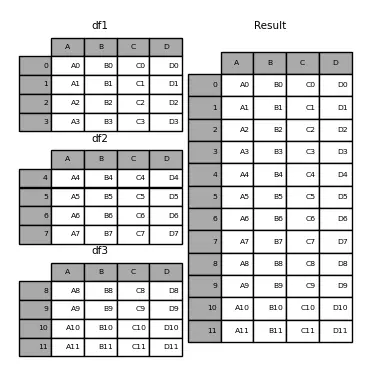
To concatenate multiple DataFrames we use the concat() method, where a list of the DataFrames to be joined is passed.
InputPythondataframe1 = pd.DataFrame({"A": ["A0", "A1", "A2", "A3"],"B": ["B0", "B1", "B2", "B3"],"C": ["C0", "C1", "C2", "C3"],"D": ["D0", "D1", "D2", "D3"],})dataframe2 = pd.DataFrame({"A": ["A4", "A5", "A6", "A7"],"B": ["B4", "B5", "B6", "B7"],"C": ["C4", "C5", "C6", "C7"],"D": ["D4", "D5", "D6", "D7"],})dataframe3 = pd.DataFrame({"A": ["A8", "A9", "A10", "A11"],"B": ["B8", "B9", "B10", "B11"],"C": ["C8", "C9", "C10", "C11"],"D": ["D8", "D9", "D10", "D11"],})dataframe = pd.concat([dataframe1, dataframe2, dataframe3])print(f"dataframe1: {dataframe1}")print(f"dataframe2: {dataframe2}")print(f"dataframe3: {dataframe3}")print(f" dataframe: {dataframe}")Copied
dataframe1:A B C D0 A0 B0 C0 D01 A1 B1 C1 D12 A2 B2 C2 D23 A3 B3 C3 D3dataframe2:A B C D0 A4 B4 C4 D41 A5 B5 C5 D52 A6 B6 C6 D63 A7 B7 C7 D7dataframe3:A B C D0 A8 B8 C8 D81 A9 B9 C9 D92 A10 B10 C10 D103 A11 B11 C11 D11dataframe:A B C D0 A0 B0 C0 D01 A1 B1 C1 D12 A2 B2 C2 D23 A3 B3 C3 D30 A4 B4 C4 D41 A5 B5 C5 D52 A6 B6 C6 D63 A7 B7 C7 D70 A8 B8 C8 D81 A9 B9 C9 D92 A10 B10 C10 D103 A11 B11 C11 D11
As can be seen, the indices 0, 1, 2, and 3 are repeated because each dataframe has those indices. To prevent this, you should use the parameter ignore_index=True.
InputPythondataframe = pd.concat([dataframe1, dataframe2, dataframe3], ignore_index=True)print(f"dataframe1: {dataframe1}")print(f"dataframe2: {dataframe2}")print(f"dataframe3: {dataframe3}")print(f" dataframe: {dataframe}")Copied
dataframe1:A B C D0 A0 B0 C0 D01 A1 B1 C1 D12 A2 B2 C2 D23 A3 B3 C3 D3dataframe2:A B C D0 A4 B4 C4 D41 A5 B5 C5 D52 A6 B6 C6 D63 A7 B7 C7 D7dataframe3:A B C D0 A8 B8 C8 D81 A9 B9 C9 D92 A10 B10 C10 D103 A11 B11 C11 D11dataframe:A B C D0 A0 B0 C0 D01 A1 B1 C1 D12 A2 B2 C2 D23 A3 B3 C3 D34 A4 B4 C4 D45 A5 B5 C5 D56 A6 B6 C6 D67 A7 B7 C7 D78 A8 B8 C8 D89 A9 B9 C9 D910 A10 B10 C10 D1011 A11 B11 C11 D11
If the concatenation was intended to be performed along the columns, the variable axis=1 should have been used.
InputPythondataframe = pd.concat([dataframe1, dataframe2, dataframe3], axis=1)print(f"dataframe1: {dataframe1}")print(f"dataframe2: {dataframe2}")print(f"dataframe3: {dataframe3}")print(f" dataframe: {dataframe}")Copied
dataframe1:A B C D0 A0 B0 C0 D01 A1 B1 C1 D12 A2 B2 C2 D23 A3 B3 C3 D3dataframe2:A B C D0 A4 B4 C4 D41 A5 B5 C5 D52 A6 B6 C6 D63 A7 B7 C7 D7dataframe3:A B C D0 A8 B8 C8 D81 A9 B9 C9 D92 A10 B10 C10 D103 A11 B11 C11 D11dataframe:A B C D A B C D A B C D0 A0 B0 C0 D0 A4 B4 C4 D4 A8 B8 C8 D81 A1 B1 C1 D1 A5 B5 C5 D5 A9 B9 C9 D92 A2 B2 C2 D2 A6 B6 C6 D6 A10 B10 C10 D103 A3 B3 C3 D3 A7 B7 C7 D7 A11 B11 C11 D11
12.1.1. Intersection of Concatenation
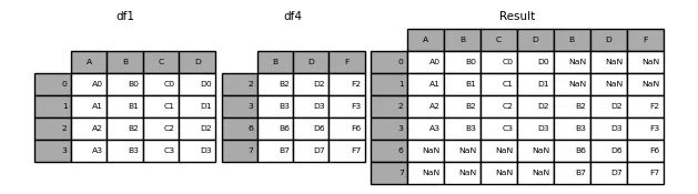
There are two ways to perform the concatenation, either taking all the indices from the DataFrames or only those that match. This is determined by the join variable, which accepts the values 'outer' (default) (takes all indices) or 'inner' (only those that match).
Let's see an example of 'outer'
InputPythondataframe1 = pd.DataFrame({"A": ["A0", "A1", "A2", "A3"],"B": ["B0", "B1", "B2", "B3"],"C": ["C0", "C1", "C2", "C3"],"D": ["D0", "D1", "D2", "D3"],},index=[0, 1, 2, 3])dataframe4 = pd.DataFrame({"B": ["B2", "B3", "B6", "B7"],"D": ["D2", "D3", "D6", "D7"],"F": ["F2", "F3", "F6", "F7"],},index=[2, 3, 6, 7])dataframe = pd.concat([dataframe1, dataframe4], axis=1)print(f"dataframe1: {dataframe1}")print(f"dataframe2: {dataframe4}")print(f" dataframe: {dataframe}")Copied
dataframe1:A B C D0 A0 B0 C0 D01 A1 B1 C1 D12 A2 B2 C2 D23 A3 B3 C3 D3dataframe2:B D F2 B2 D2 F23 B3 D3 F36 B6 D6 F67 B7 D7 F7dataframe:A B C D B D F0 A0 B0 C0 D0 NaN NaN NaN1 A1 B1 C1 D1 NaN NaN NaN2 A2 B2 C2 D2 B2 D2 F23 A3 B3 C3 D3 B3 D3 F36 NaN NaN NaN NaN B6 D6 F67 NaN NaN NaN NaN B7 D7 F7
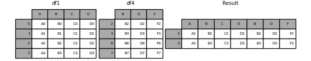
Let's see an example of 'inner'
InputPythondataframe = pd.concat([dataframe1, dataframe4], axis=1, join="inner")print(f"dataframe1: {dataframe1}")print(f"dataframe2: {dataframe4}")print(f" dataframe: {dataframe}")Copied
dataframe1:A B C D0 A0 B0 C0 D01 A1 B1 C1 D12 A2 B2 C2 D23 A3 B3 C3 D3dataframe2:B D F2 B2 D2 F23 B3 D3 F36 B6 D6 F67 B7 D7 F7dataframe:A B C D B D F2 A2 B2 C2 D2 B2 D2 F23 A3 B3 C3 D3 B3 D3 F3
12.2. Merge of DataFrames
We previously created a new dataframe by merging several dataframes. Now we can complete one dataframe with another using merge, passing the parameter on to specify which column should be used for the merge.
InputPythondataframe1 = pd.DataFrame({"Key": ["K0", "K1", "K2", "K3"],"A": ["A0", "A1", "A2", "A3"],"B": ["B0", "B1", "B2", "B3"],})dataframe2 = pd.DataFrame({"Key": ["K0", "K1", "K2", "K3"],"C": ["C0", "C1", "C2", "C3"],"D": ["D0", "D1", "D2", "D3"],})dataframe = dataframe1.merge(dataframe2, on="Key")print(f"dataframe1: {dataframe1}")print(f"dataframe2: {dataframe2}")print(f" dataframe: {dataframe}")Copied
dataframe1:Key A B0 K0 A0 B01 K1 A1 B12 K2 A2 B23 K3 A3 B3dataframe2:Key C D0 K0 C0 D01 K1 C1 D12 K2 C2 D23 K3 C3 D3dataframe:Key A B C D0 K0 A0 B0 C0 D01 K1 A1 B1 C1 D12 K2 A2 B2 C2 D23 K3 A3 B3 C3 D3
In this case, both dataframes had a key with the same name (Key), but if we have dataframes where their keys are named differently, we can use the left_on and right_on parameters.
InputPythondataframe1 = pd.DataFrame({"Key1": ["K0", "K1", "K2", "K3"],"A": ["A0", "A1", "A2", "A3"],"B": ["B0", "B1", "B2", "B3"],})dataframe2 = pd.DataFrame({"Key2": ["K0", "K1", "K2", "K3"],"C": ["C0", "C1", "C2", "C3"],"D": ["D0", "D1", "D2", "D3"],})dataframe = dataframe1.merge(dataframe2, left_on="Key1", right_on="Key2")print(f"dataframe1: {dataframe1}")print(f"dataframe2: {dataframe2}")print(f" dataframe: {dataframe}")Copied
dataframe1:Key1 A B0 K0 A0 B01 K1 A1 B12 K2 A2 B23 K3 A3 B3dataframe2:Key2 C D0 K0 C0 D01 K1 C1 D12 K2 C2 D23 K3 C3 D3dataframe:Key1 A B Key2 C D0 K0 A0 B0 K0 C0 D01 K1 A1 B1 K1 C1 D12 K2 A2 B2 K2 C2 D23 K3 A3 B3 K3 C3 D3
In the case where one of the keys does not match, the merge will not be performed on that key.
InputPythondataframe1 = pd.DataFrame({"Key1": ["K0", "K1", "K2", "K3"],"A": ["A0", "A1", "A2", "A3"],"B": ["B0", "B1", "B2", "B3"],})dataframe2 = pd.DataFrame({"Key2": ["K0", "K1", "K2", np.nan],"C": ["C0", "C1", "C2", "C3"],"D": ["D0", "D1", "D2", "D3"],})dataframe = dataframe1.merge(dataframe2, left_on="Key1", right_on="Key2")print(f"dataframe1: {dataframe1}")print(f"dataframe2: {dataframe2}")print(f" dataframe: {dataframe}")Copied
dataframe1:Key1 A B0 K0 A0 B01 K1 A1 B12 K2 A2 B23 K3 A3 B3dataframe2:Key2 C D0 K0 C0 D01 K1 C1 D12 K2 C2 D23 NaN C3 D3dataframe:Key1 A B Key2 C D0 K0 A0 B0 K0 C0 D01 K1 A1 B1 K1 C1 D12 K2 A2 B2 K2 C2 D2
To change this behavior, we can use the how parameter, which by default has the value inner, but we can pass it the values left, right, and outer.
InputPythondataframe1 = pd.DataFrame({"Key1": ["K0", "K1", "K2", "K3"],"A": ["A0", "A1", "A2", "A3"],"B": ["B0", "B1", "B2", "B3"],})dataframe2 = pd.DataFrame({"Key2": ["K0", "K1", "K2", np.nan],"C": ["C0", "C1", "C2", "C3"],"D": ["D0", "D1", "D2", "D3"],})dataframe_inner = dataframe1.merge(dataframe2, left_on="Key1", right_on="Key2", how="inner")dataframe_left = dataframe1.merge(dataframe2, left_on="Key1", right_on="Key2", how="left")dataframe_right = dataframe1.merge(dataframe2, left_on="Key1", right_on="Key2", how="right")dataframe_outer = dataframe1.merge(dataframe2, left_on="Key1", right_on="Key2", how="outer")print(f"dataframe1: {dataframe1}")print(f"dataframe2: {dataframe2}")print(f" dataframe inner: {dataframe_inner}")print(f" dataframe left: {dataframe_left}")print(f" dataframe right: {dataframe_right}")print(f" dataframe outer: {dataframe_outer}")Copied
dataframe1:Key1 A B0 K0 A0 B01 K1 A1 B12 K2 A2 B23 K3 A3 B3dataframe2:Key2 C D0 K0 C0 D01 K1 C1 D12 K2 C2 D23 NaN C3 D3dataframe inner:Key1 A B Key2 C D0 K0 A0 B0 K0 C0 D01 K1 A1 B1 K1 C1 D12 K2 A2 B2 K2 C2 D2dataframe left:Key1 A B Key2 C D0 K0 A0 B0 K0 C0 D01 K1 A1 B1 K1 C1 D12 K2 A2 B2 K2 C2 D23 K3 A3 B3 NaN NaN NaNdataframe right:Key1 A B Key2 C D0 K0 A0 B0 K0 C0 D01 K1 A1 B1 K1 C1 D12 K2 A2 B2 K2 C2 D23 NaN NaN NaN NaN C3 D3dataframe outer:Key1 A B Key2 C D0 K0 A0 B0 K0 C0 D01 K1 A1 B1 K1 C1 D12 K2 A2 B2 K2 C2 D23 K3 A3 B3 NaN NaN NaN4 NaN NaN NaN NaN C3 D3
As can be seen, when left is chosen, only the values from the left dataframe are added, and when right is chosen, the values from the right dataframe are added.
12.3. Join of dataframes
The last tool for joining dataframes is join. It is similar to merge, except that instead of looking for similarities based on specified columns, it looks for them based on the indices.
InputPythondataframe1 = pd.DataFrame({"A": ["A0", "A1", "A2", "A3"],"B": ["B0", "B1", "B2", "B3"],},index=["K0", "K1", "K2", "K3"])dataframe2 = pd.DataFrame({"C": ["C0", "C1", "C2", "C3"],"D": ["D0", "D1", "D2", "D3"],},index=["K0", "K1", "K2", "K3"])dataframe = dataframe1.join(dataframe2)print(f"dataframe1: {dataframe1}")print(f"dataframe2: {dataframe2}")print(f" dataframe: {dataframe}")Copied
dataframe1:A BK0 A0 B0K1 A1 B1K2 A2 B2K3 A3 B3dataframe2:C DK0 C0 D0K1 C1 D1K2 C2 D2K3 C3 D3dataframe:A B C DK0 A0 B0 C0 D0K1 A1 B1 C1 D1K2 A2 B2 C2 D2K3 A3 B3 C3 D3
In this case, the indices are the same, but when they are different we can specify how to join the dataframes using the how parameter, which by default has the value inner, but can also have the values left, right, or outer.
InputPythondataframe1 = pd.DataFrame({"A": ["A0", "A1", "A2", "A3"],"B": ["B0", "B1", "B2", "B3"],},index=["K0", "K1", "K2", "K3"])dataframe2 = pd.DataFrame({"C": ["C0", "C2", "C3", "C4"],"D": ["D0", "D2", "D3", "D4"],},index=["K0", "K2", "K3", "K4"])dataframe_inner = dataframe1.join(dataframe2, how="inner")dataframe_left = dataframe1.join(dataframe2, how="left")dataframe_right = dataframe1.join(dataframe2, how="right")dataframe_outer = dataframe1.join(dataframe2, how="outer")print(f"dataframe1: {dataframe1}")print(f"dataframe2: {dataframe2}")print(f" dataframe inner: {dataframe_inner}")print(f" dataframe left: {dataframe_left}")print(f" dataframe rigth: {dataframe_right}")print(f" dataframe outer: {dataframe_outer}")Copied
dataframe1:A BK0 A0 B0K1 A1 B1K2 A2 B2K3 A3 B3dataframe2:C DK0 C0 D0K2 C2 D2K3 C3 D3K4 C4 D4dataframe:A B C DK0 A0 B0 C0 D0K2 A2 B2 C2 D2K3 A3 B3 C3 D3dataframe:A B C DK0 A0 B0 C0 D0K1 A1 B1 NaN NaNK2 A2 B2 C2 D2K3 A3 B3 C3 D3dataframe:A B C DK0 A0 B0 C0 D0K2 A2 B2 C2 D2K3 A3 B3 C3 D3K4 NaN NaN C4 D4dataframe:A B C DK0 A0 B0 C0 D0K1 A1 B1 NaN NaNK2 A2 B2 C2 D2K3 A3 B3 C3 D3K4 NaN NaN C4 D4
13. Missing data (NaN)
In a DataFrame there can be some missing data, Pandas represents them as np.nan
InputPythondiccionario = {"uno": pd.Series([1.0, 2.0, 3.0]),"dos": pd.Series([4.0, 5.0, 6.0, 7.0])}dataframe = pd.DataFrame(diccionario)dataframeCopied
uno dos0 1.0 4.01 2.0 5.02 3.0 6.03 NaN 7.0
13.1. Removal of Rows with Missing Data
To avoid having rows with missing data, these can be removed.
InputPythondataframe.dropna(how="any")Copied
uno dos0 1.0 4.01 2.0 5.02 3.0 6.0
13.2. Dropping Columns with Missing Data
InputPythondataframe.dropna(axis=1, how='any')Copied
dos0 4.01 5.02 6.03 7.0
13.3. Boolean mask with missing positions
InputPythonpd.isna(dataframe)Copied
uno dos0 False False1 False False2 False False3 True False
13.4. Filling Missing Data
InputPythondataframe.fillna(value=5.5, inplace=True)dataframeCopied
uno dos0 1.0 4.01 2.0 5.02 3.0 6.03 5.5 7.0
Tip: By setting the variable
inplace=True, theDataFramebeing operated on is modified, so there's no need to writedataframe = dataframe.fillna(value=5.5)
14. Time series
Pandas offers the possibility of working with time series. For example, we create a Series of 100 random data points every second starting from 01/01/2021
InputPythonindices = pd.date_range("1/1/2021", periods=100, freq="S")datos = np.random.randint(0, 500, len(indices))serie_temporal = pd.Series(datos, index=indices)serie_temporalCopied
2021-01-01 00:00:00 2412021-01-01 00:00:01 142021-01-01 00:00:02 1902021-01-01 00:00:03 4072021-01-01 00:00:04 94...2021-01-01 00:01:35 2752021-01-01 00:01:36 562021-01-01 00:01:37 4482021-01-01 00:01:38 1512021-01-01 00:01:39 316Freq: S, Length: 100, dtype: int64
This Pandas functionality is very powerful, for example, we can have a dataset at certain hours of one time zone and change them to another time zone.
InputPythonhoras = pd.date_range("3/6/2021 00:00", periods=10, freq="H")datos = np.random.randn(len(horas))serie_horaria = pd.Series(datos, horas)serie_horariaCopied
2021-03-06 00:00:00 -0.8535242021-03-06 01:00:00 -1.3553722021-03-06 02:00:00 -1.2675032021-03-06 03:00:00 -1.1557872021-03-06 04:00:00 0.7309352021-03-06 05:00:00 1.4359572021-03-06 06:00:00 0.4609122021-03-06 07:00:00 0.7234512021-03-06 08:00:00 -0.8533372021-03-06 09:00:00 0.456359Freq: H, dtype: float64
We locate the data in a time zone
InputPythonserie_horaria_utc = serie_horaria.tz_localize("UTC")serie_horaria_utcCopied
2021-03-06 00:00:00+00:00 -0.8535242021-03-06 01:00:00+00:00 -1.3553722021-03-06 02:00:00+00:00 -1.2675032021-03-06 03:00:00+00:00 -1.1557872021-03-06 04:00:00+00:00 0.7309352021-03-06 05:00:00+00:00 1.4359572021-03-06 06:00:00+00:00 0.4609122021-03-06 07:00:00+00:00 0.7234512021-03-06 08:00:00+00:00 -0.8533372021-03-06 09:00:00+00:00 0.456359Freq: H, dtype: float64
And now we can change them to another use
InputPythonserie_horaria_US = serie_horaria_utc.tz_convert("US/Eastern")serie_horaria_USCopied
2021-03-05 19:00:00-05:00 -0.8535242021-03-05 20:00:00-05:00 -1.3553722021-03-05 21:00:00-05:00 -1.2675032021-03-05 22:00:00-05:00 -1.1557872021-03-05 23:00:00-05:00 0.7309352021-03-06 00:00:00-05:00 1.4359572021-03-06 01:00:00-05:00 0.4609122021-03-06 02:00:00-05:00 0.7234512021-03-06 03:00:00-05:00 -0.8533372021-03-06 04:00:00-05:00 0.456359Freq: H, dtype: float64
15. Categorical Data
Pandas offers the possibility of adding categorical data in a DataFrame. Suppose the following DataFrame
InputPythondataframe = pd.DataFrame({"id": [1, 2, 3, 4, 5, 6], "raw_grade": ["a", "b", "b", "a", "a", "e"]})dataframeCopied
id raw_grade0 1 a1 2 b2 3 b3 4 a4 5 a5 6 e
We can convert the data in the raw_grade column to categorical data using the astype() method.
InputPythondataframe['grade'] = dataframe["raw_grade"].astype("category")dataframeCopied
id raw_grade grade0 1 a a1 2 b b2 3 b b3 4 a a4 5 a a5 6 e e
The columns raw_grade and grade seem identical, but if we look at the information of the DataFrame we can see that this is not the case.
InputPythondataframe.info()Copied
<class 'pandas.core.frame.DataFrame'>RangeIndex: 6 entries, 0 to 5Data columns (total 3 columns):# Column Non-Null Count Dtype--- ------ -------------- -----0 id 6 non-null int641 raw_grade 6 non-null object2 grade 6 non-null categorydtypes: category(1), int64(1), object(1)memory usage: 334.0+ bytes
It can be seen that the column grade is of categorical type
We can see the categories of categorical data types through the method cat.categories()
InputPythondataframe["grade"].cat.categoriesCopied
Index(['a', 'b', 'e'], dtype='object')
We can also rename the categories using the same method, but by providing a list with the new categories.
InputPythondataframe["grade"].cat.categories = ["very good", "good", "very bad"]dataframeCopied
id raw_grade grade0 1 a very good1 2 b good2 3 b good3 4 a very good4 5 a very good5 6 e very bad
Pandas gives us the possibility to numerically encode categorical data using the get_dummies method.
InputPythonpd.get_dummies(dataframe["grade"])Copied
very good good very bad0 1 0 01 0 1 02 0 1 03 1 0 04 1 0 05 0 0 1
16. Groupby
We can group the dataframes by values from one of the columns. Let's reload the dataframe with the value of houses in California.
InputPythoncalifornia_housing_train = pd.read_csv("https://raw.githubusercontent.com/maximofn/portafolio/main/posts/california_housing_train.csv")california_housing_train.head()Copied
longitude latitude housing_median_age total_rooms total_bedrooms \0 -114.31 34.19 15.0 5612.0 1283.01 -114.47 34.40 19.0 7650.0 1901.02 -114.56 33.69 17.0 720.0 174.03 -114.57 33.64 14.0 1501.0 337.04 -114.57 33.57 20.0 1454.0 326.0population households median_income median_house_value0 1015.0 472.0 1.4936 66900.01 1129.0 463.0 1.8200 80100.02 333.0 117.0 1.6509 85700.03 515.0 226.0 3.1917 73400.04 624.0 262.0 1.9250 65500.0
Now we can group the data by one of the columns, for example, let's group the houses based on the number of years and see how many houses there are of each age with count
InputPythoncalifornia_housing_train.groupby("housing_median_age").count().head()Copied
longitude latitude total_rooms total_bedrooms \housing_median_age1.0 2 2 2 22.0 49 49 49 493.0 46 46 46 464.0 161 161 161 1615.0 199 199 199 199population households median_income median_house_valuehousing_median_age1.0 2 2 2 22.0 49 49 49 493.0 46 46 46 464.0 161 161 161 1615.0 199 199 199 199
As we can see in all the columns, we get the same value, which is the number of houses that have a certain age, but we can find out the average value of each column with mean
InputPythoncalifornia_housing_train.groupby("housing_median_age").mean().head()Copied
longitude latitude total_rooms total_bedrooms \housing_median_age1.0 -121.465000 37.940000 2158.000000 335.5000002.0 -119.035306 35.410816 5237.102041 871.4489803.0 -118.798478 35.164783 6920.326087 1190.8260874.0 -118.805093 34.987764 6065.614907 1068.1925475.0 -118.789497 35.095327 4926.261307 910.924623population households median_income \housing_median_age1.0 637.000000 190.000000 4.7568002.0 2005.224490 707.122449 5.0742373.0 2934.673913 1030.413043 5.5720134.0 2739.956522 964.291925 5.1960555.0 2456.979899 826.768844 4.732460median_house_valuehousing_median_age1.0 190250.0000002.0 229438.8367353.0 239450.0434784.0 230054.1055905.0 211035.708543
We can obtain several measures for each age using the agg (aggregation) command, passing it the measures we want through a list. For example, let's look at the minimum, maximum, and mean of each column for each age:
InputPythoncalifornia_housing_train.groupby("housing_median_age").agg(['min', 'max', 'mean']).head()Copied
longitude latitude \min max mean min max meanhousing_median_age1.0 -122.00 -120.93 -121.465000 37.65 38.23 37.9400002.0 -122.51 -115.80 -119.035306 33.16 40.58 35.4108163.0 -122.33 -115.60 -118.798478 32.87 38.77 35.1647834.0 -122.72 -116.76 -118.805093 32.65 39.00 34.9877645.0 -122.55 -115.55 -118.789497 32.55 40.60 35.095327total_rooms total_bedrooms ... \min max mean min ...housing_median_age ...1.0 2062.0 2254.0 2158.000000 328.0 ...2.0 96.0 21897.0 5237.102041 18.0 ...3.0 475.0 21060.0 6920.326087 115.0 ...4.0 2.0 37937.0 6065.614907 2.0 ...5.0 111.0 25187.0 4926.261307 21.0 ...population households median_income \mean min max mean minhousing_median_age1.0 637.000000 112.0 268.0 190.000000 4.2500...5.0 12.6320 4.732460 50000.0 500001.0meanhousing_median_age1.0 190250.0000002.0 229438.8367353.0 239450.0434784.0 230054.1055905.0 211035.708543[5 rows x 24 columns]
We can specify on which columns we want to perform certain calculations by passing a dictionary, where the keys will be the columns on which we want to perform calculations and the values will be lists with the calculations.
InputPythoncalifornia_housing_train.groupby("housing_median_age").agg({'total_rooms': ['min', 'max', 'mean'], 'total_bedrooms': ['min', 'max', 'mean', 'median']}).head()Copied
total_rooms total_bedrooms \min max mean min maxhousing_median_age1.0 2062.0 2254.0 2158.000000 328.0 343.02.0 96.0 21897.0 5237.102041 18.0 3513.03.0 475.0 21060.0 6920.326087 115.0 3559.04.0 2.0 37937.0 6065.614907 2.0 5471.05.0 111.0 25187.0 4926.261307 21.0 4386.0mean medianhousing_median_age1.0 335.500000 335.52.0 871.448980 707.03.0 1190.826087 954.04.0 1068.192547 778.05.0 910.924623 715.0
We can group by more than one column, for this, we have to pass the columns in a list
InputPythoncalifornia_housing_train.groupby(["housing_median_age", "total_bedrooms"]).mean()Copied
longitude latitude total_rooms \housing_median_age total_bedrooms1.0 328.0 -120.93 37.65 2254.0343.0 -122.00 38.23 2062.02.0 18.0 -115.80 33.26 96.035.0 -121.93 37.78 227.055.0 -117.27 33.93 337.0... ... ... ...52.0 1360.0 -118.35 34.06 3446.01535.0 -122.41 37.80 3260.01944.0 -118.25 34.05 2806.02509.0 -122.41 37.79 6016.02747.0 -122.41 37.79 5783.0population households median_income \housing_median_age total_bedrooms1.0 328.0 402.0 112.0 4.2500343.0 872.0 268.0 5.26362.0 18.0 30.0 16.0 5.337435.0 114.0 49.0 3.159155.0 115.0 49.0 3.1042... ... ... ...52.0 1360.0 1768.0 1245.0 2.47221535.0 3260.0 1457.0 0.90001944.0 2232.0 1605.0 0.67752509.0 3436.0 2119.0 2.51662747.0 4518.0 2538.0 1.7240median_house_valuehousing_median_age total_bedrooms1.0 328.0 189200.0343.0 191300.02.0 18.0 47500.035.0 434700.055.0 164800.0... ...52.0 1360.0 500001.01535.0 500001.01944.0 350000.02509.0 275000.02747.0 225000.0[13394 rows x 7 columns]
17. Graphics
Pandas offers the possibility of representing the data in our DataFrames in charts to obtain a better representation of it. For this, it uses the matplotlib library, which we will cover in the next post.
17.1. Basic Graph
To represent the data in a chart, the easiest way is to use the plot() method.
InputPythonserie = pd.Series(np.random.randn(1000), index=pd.date_range("1/1/2000", periods=1000))serie = serie.cumsum()serie.plot()Copied
<matplotlib.axes._subplots.AxesSubplot at 0x7fc5666b9990>
<Figure size 432x288 with 1 Axes>
In the case of having a DataFrame, the plot() method will represent each of the columns of the DataFrame
InputPythondataframe = pd.DataFrame(np.random.randn(1000, 4), index=ts.index, columns=["A", "B", "C", "D"])dataframe = dataframe.cumsum()dataframe.plot()Copied
<matplotlib.axes._subplots.AxesSubplot at 0x7fc5663ce610>
<Figure size 432x288 with 1 Axes>
17.2. Vertical Bar Chart
There are more methods to create charts, such as the vertical bar chart using plot.bar()
InputPythondataframe = pd.DataFrame(np.random.rand(10, 4), columns=["a", "b", "c", "d"])dataframe.plot.bar()Copied
<Figure size 432x288 with 1 Axes>
If we want to stack the bars, we indicate this through the variable stacked=True
InputPythondataframe.plot.bar(stacked=True)Copied
<matplotlib.axes._subplots.AxesSubplot at 0x7fc56265c5d0>
<Figure size 432x288 with 1 Axes>
17.3. Horizontal Bar Chart
To create a horizontal bar chart we use plot.barh()
InputPythondataframe.plot.barh()Copied
<matplotlib.axes._subplots.AxesSubplot at 0x7fc56247fa10>
<Figure size 432x288 with 1 Axes>
If we want to stack the bars, we indicate this through the variable stacked=True
InputPythondataframe.plot.barh(stacked=True)Copied
<matplotlib.axes._subplots.AxesSubplot at 0x7fc562d1d2d0>
<Figure size 432x288 with 1 Axes>
17.4. Histogram
To create a histogram we use plot.hist()
InputPythondataframe = pd.DataFrame({"a": np.random.randn(1000) + 1,"b": np.random.randn(1000),"c": np.random.randn(1000) - 1,})dataframe.plot.hist(alpha=0.5)Copied
<matplotlib.axes._subplots.AxesSubplot at 0x7fc5650711d0>
<Figure size 432x288 with 1 Axes>
If we want to stack the bars, we indicate this through the variable stacked=True
InputPythondataframe.plot.hist(alpha=0.5, stacked=True)Copied
<matplotlib.axes._subplots.AxesSubplot at 0x7fc5625779d0>
<Figure size 432x288 with 1 Axes>
If we want to add more columns, that is, if we want the histogram to be more informative or accurate, we indicate this through the bins variable.
InputPythondataframe.plot.hist(alpha=0.5, stacked=True, bins=20)Copied
<matplotlib.axes._subplots.AxesSubplot at 0x7fc562324990>
<Figure size 432x288 with 1 Axes>
17.5. Candlestick Diagrams
To create a candlestick chart we use plot.box()
InputPythondataframe = pd.DataFrame(np.random.rand(10, 5), columns=["A", "B", "C", "D", "E"])dataframe.plot.box()Copied
<matplotlib.axes._subplots.AxesSubplot at 0x7fc56201a410>
<Figure size 432x288 with 1 Axes>
17.6. Area Charts
To create an area chart we use plot.area()
InputPythondataframe.plot.area()Copied
<matplotlib.axes._subplots.AxesSubplot at 0x7fc561e9ca50>
<Figure size 432x288 with 1 Axes>
17.7. Scatter plot
To create a scatter plot we use plot.scatter(), where you need to specify the x and y variables of the plot.
InputPythondataframe.plot.scatter(x='A', y='B')Copied
<matplotlib.axes._subplots.AxesSubplot at 0x7fc561e2ff10>
<Figure size 432x288 with 1 Axes>
17.8. Hexagonal Container Plot
To create a hexagonal bin plot we use plot.hexbin(), where you need to specify the x and y variables of the plot and the mesh size using gridsize.
InputPythondataframe = pd.DataFrame(np.random.randn(1000, 2), columns=["a", "b"])dataframe["b"] = dataframe["b"] + np.arange(1000)dataframe.plot.hexbin(x="a", y="b", gridsize=25)Copied
<matplotlib.axes._subplots.AxesSubplot at 0x7fc561cdded0>
<Figure size 432x288 with 2 Axes>