Transformers - from top to the bottom

In this post we are going to look at how Transformers work from top to bottom.

This notebook has been automatically translated to make it accessible to more people, please let me know if you see any typos.

Transformer as a black box

The transformer architecture was created for the translation problem, so let's explain it for that problem.

Imagine the transformer as a black box, which takes a sentence in one language and outputs the same sentence translated into another language.

Tokenization

But as we have seen in the tokens post, language models do not understand words as we do, they need numbers to be able to perform operations. So the original language sentence has to be converted to tokens by a tokenizer, and at the output we need a detokenizer to convert the output tokens to words

So the tokenizer creates a sequence of $n_{input-tokens}$ tokens, and the detokenizer receives a sequence of $n_{output-tokens}$ tokens.

Input embeddings

In the embeddings post we saw that embeddings are a way of representing words in a vector space. So the input tokens are passed through an embeddings layer to convert them into vectors.

In a quick summary, the embedding process consists of converting a sequence of numbers (tokens) into a sequence of vectors. So a new vector space is created in which words that have semantic similarity will be close to each other.

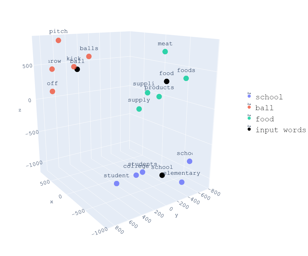
If we had $n_{input-tokens}$ tokens, we now have $n_{input-tokens}$ vectors. Each of those vectors has a length of $d_{model}$. That is, each token is converted to a vector representing that token in a $d_{model}$$-dimensional vector space. Therefore after passing through the embeddings layer, the sequence of $n_{input-tokens}$ tokens becomes an array of ($n_{input-tokens}$$ x $d_{model}$).

Encoder - decoder

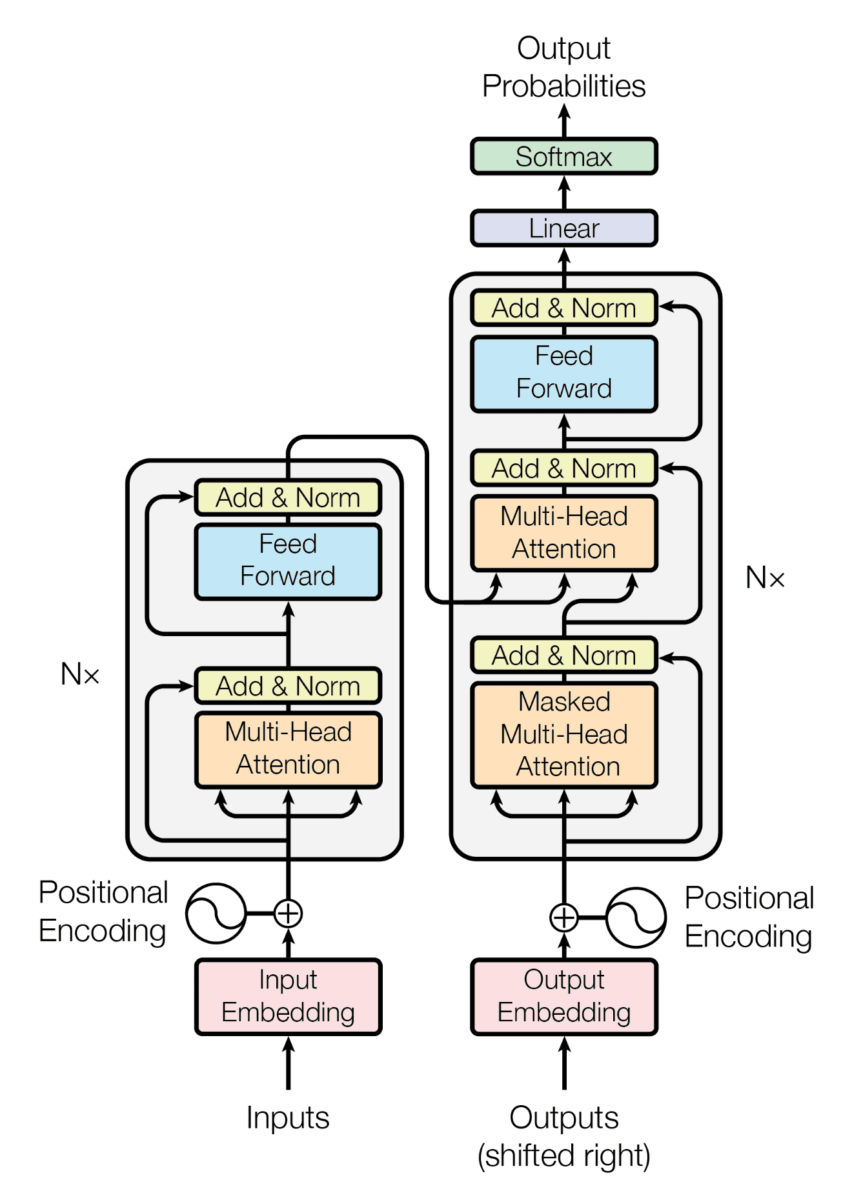
We have seen the transformer acting as a black box, but in reality the transformer is an architecture that is composed of two parts, an encoder and a decoder.

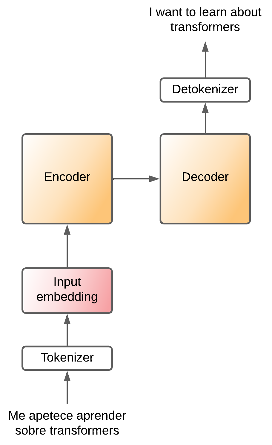
The encoder is in charge of compressing the information of the input sentence, it creates a latent space where the information of the input sentence is compressed. Then, that compressed information enters the decoder, which knows how to convert that compressed information into a phrase of the output language.

And how does the decoder convert this compressed information into a sentence of the output language? Well, token by token. To understand it better, let's forget about the output tokens for a moment, let's imagine that we have this architecture

Transformer - encoder-decoder (no detokenizer)](https://pub-fb664c455eca46a2ba762a065ac900f7.r2.dev/Transformer-encoder-decoder-no-detokenizer.webp)

That is, the original language sentence is converted to tokens, these tokens are converted to embeddings, which enter the encoder, which compresses the information, the decoder takes it and converts it into words of the output language.

So the decoder generates a new word at the output at each step.

But how does the decoder know which word to generate each time? Because it is being passed the phrase it has already translated, and at each step it generates the next word. That is, at each step the decoder receives the phrase it has translated so far, and generates the next word.

But still, how does it know to generate the first word? Because it is passed a special word that means "start translating", and from there it generates the following words.

And finally, how does the transformer know that it has to stop generating words? Because when it finishes translating it generates a special word meaning "end of translation", which when it re-enters the transformer makes it not generate any more words.

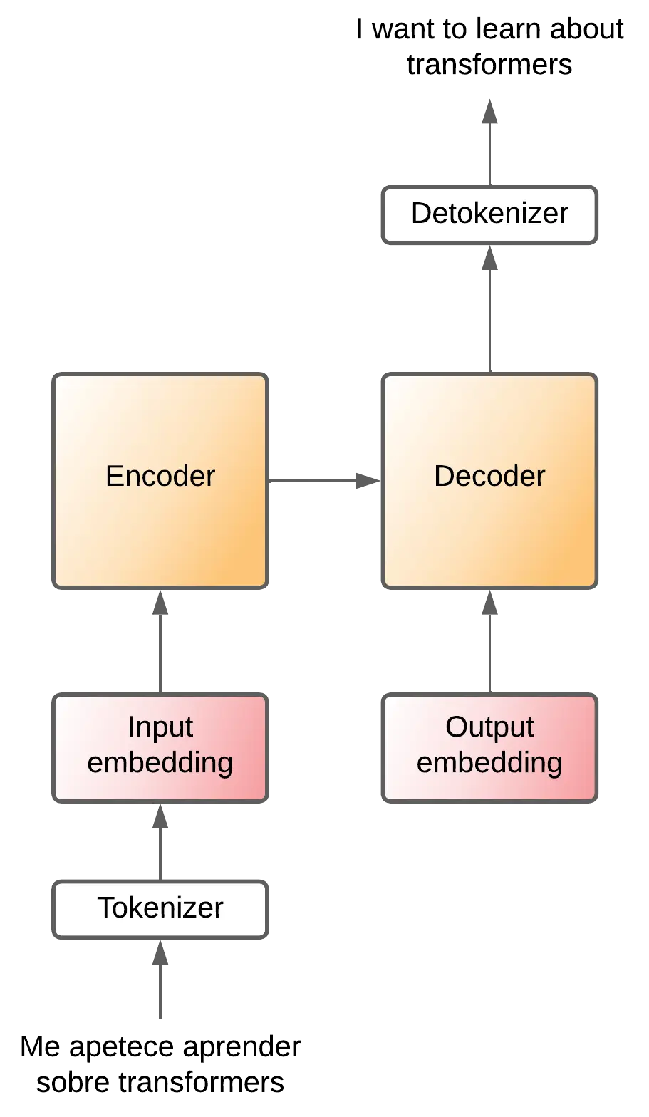
Now that we have understood it in words, which is simpler, let's put the detokenizer back to the output

Therefore the decoder will be generating tokens. To know that it has to start a sentence a special token commonly called SOS (Start Of Sentence) is inserted, and to know that it has to end it generates another special token commonly called EOS (End Of Sentence).

And just like the encoder, the input token has to go through an embedding layer to convert the tokens into vector representations.

Assuming that each token is equivalent to one word, the translation process would be as follows

At the moment we have this architecture

Projection

We have said that the decoder receives a token that passes through the embedding layer Output embedding.

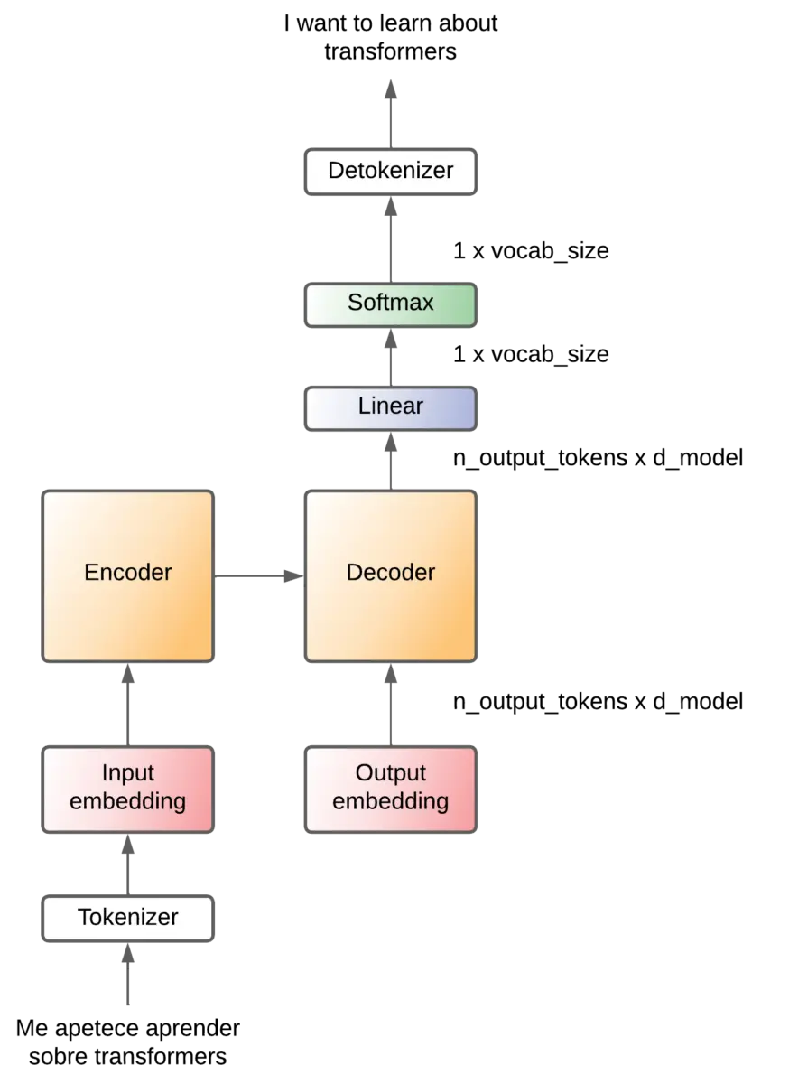
The Output decoder creates a vector for each token, so at the output of the Output decoder we have an array of ($n_{output-tokens}$ x $d_{model}$).

The decoder performs operations, but outputs an array with the same dimension. So it needs to convert that matrix into a token and it does it by means of a linear layer that generates an array with the same dimension as the possible tokens in the language to be translated (output vocabulary).

That array corresponds to the logits of each possible token, so it is then passed through a softmax layer that converts those logits into probabilities. That is, we will have the probability that each token is the next token.

Encoder and decoder x6

In the original paper they use 6 layers for the encoder and another 6 layers for the decoder. There is no reason why there should be 6, I guess they tried several values and this was the one that worked best for them.

The output of the last encoder is fed to each decoder.

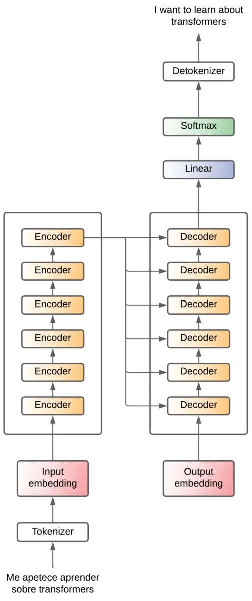
To simplify the diagram we will represent it as follows from now on

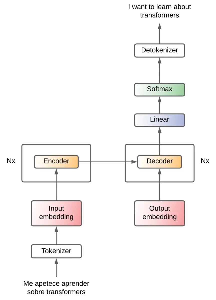
Attention - Feed forward

Let's start to see what's inside the encoder and decoder. Basically there is an attention mechanism and a feed forward layer.

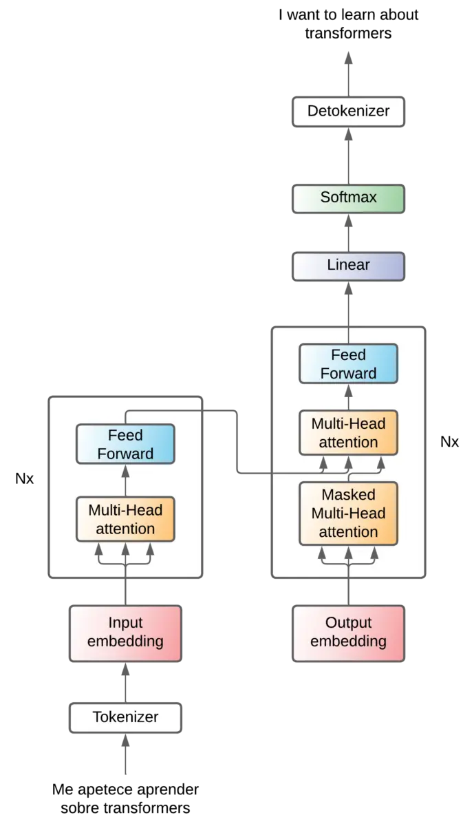
Attention

We can see that 3 arrows enter in the attention mechanisms. We will see this later when we will see in depth how the attention mechanisms work.

But for the moment we can say that they are operations that are performed in order to obtain the relationship that exists between tokens (and therefore, the relationship that exists between words).

Before transformers, recurrent neural networks were used for the translation problem, which consisted of networks that received an input token, processed it and generated another output token. Then a second token was input, processed and another token was output, and so on with all the tokens in the input sequence. The problem with these networks is that when the sentences were very long, when the last tokens were in, the network "forgot" the first tokens. For example in very long sentences, it could happen that the gender of the subject would change throughout the translated sentence. And this is because after many tokens, the network had forgotten whether the subject was masculine or feminine.

To solve this, the entire sequence is entered into the attention mechanism of the transformers and the relationships (attention) between all the tokens are calculated at once.

This is very powerful, since in a single calculation the relationship between all the tokens is obtained, no matter how long the sequence is.

While this is a great advantage and is what has led to transformers now being used in most of the best modern networks, it is also their biggest disadvantage, as the computation of the attention is very computationally expensive. It requires very large matrix multiplications.

These multiplications are performed between matrices that correspond to the embeddings of each of the tokens by themselves. That is, the matrix representing the embeddings of the tokens is multiplied by itself. In order to perform this multiplication, one of the matrices must be rotated (algebra requirements to be able to multiply matrices). So a matrix is multiplied by itself, if the input sequence has more tokens, the matrices that are multiplied are larger, one in height and one in width, so the memory needed to store these matrices grows quadratically.

So as the length of the sequences increases, the amount of memory needed to store those matrices grows quadratically. And this is a major limitation today, the amount of memory that GPUs have, which is where these multiplications are usually performed.

In the encoder, a single layer of attention is used to extract the relationships between the input tokens.

Two layers of attention are used in the decoder, one to extract the relationships between the output tokens, and the other to extract the relationships between the encoder tokens and the decoder tokens.

Feed forward

After the attention layer, the sequence enters a Feed forward layer, which has two purposes

• One is to add nonlinearities. As we have explained, attention is achieved by matrix multiplications of the tokens of the input sequences. But if no nonlinear layers are applied to a network, in the end, the whole architecture could be summarized in a few linear computations. So neural networks would not be able to solve nonlinear problems. So this layer is added to add nonlinearity.

• Another is feature extraction. Although the attention already extracts features, these are features of the relationships between the tokens. But this Feed forward layer is responsible for extracting features from the tokens themselves. That is, features are extracted from each token that are considered important for the problem being solved.

Positonal encoding

We have explained that in the attention layer the relations between the tokens are obtained, that this relation is calculated by matrix multiplications and that these multiplications are performed between the embedding matrix by itself. So in the sentences The cat eats fish and The fish eats cat, the relationship between the and cat is the same in both sentences, since the relationship is computed by matrix multiplications of the embeddings of the and cat.

However, in the first the refers to the cat, while in the second the refers to the fish. So in addition to the relationships between the words we need to have some mechanism that tells us their position in the sentence.

In the paper they propose to introduce an attention mechanism that is in charge of adding values to the embedding vectors

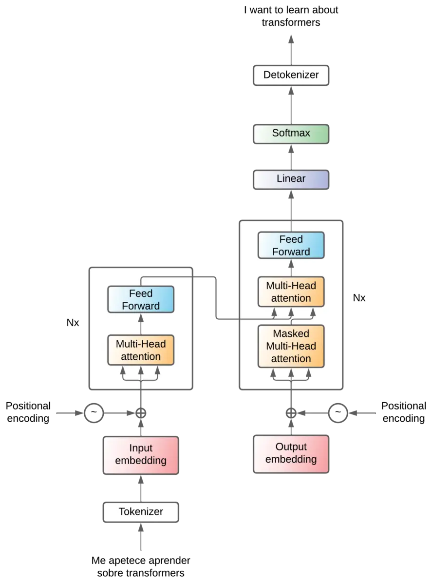
Where the formula for calculating these values is

Transformer - positional encoding (formula)](https://pub-fb664c455eca46a2ba762a065ac900f7.r2.dev/Transformer-positional-encoding-formula.webp)

As this is a bit difficult to understand, let's see what a distribution of values of the positional encoding would look like.

Transformer - positional encoding (diagram)](https://pub-fb664c455eca46a2ba762a065ac900f7.r2.dev/Transformer-positional-encoding-diagram.webp)

The first token will have the values of the first row (the bottom one) added to it, the second token the values of the second row, and so on, which causes a change in the embeddings as shown in the figure. Seen in two dimensions, the waves that are being added can be seen.

These waves cause that when attention calculations are performed, closer words have more relationship than more distant words.

But we can think one thing, if the embedding process consists of creating a vector space in which words with the same semantic meaning are close to each other, wouldn't this relationship be broken if values are added to the embeddings?

If we look again at the vector space example from before

We can see that the values go more or less from -1000 to 1000 on each axis, while the distribution graph

Transformer - positional encoding (diagram)](https://pub-fb664c455eca46a2ba762a065ac900f7.r2.dev/Transformer-positional-encoding-diagram.webp)

values range from -1 to 1, since this is the range of the sine and cosine functions.

So we are varying in a range between -1 and 1 the values of the embeddings which are two or three orders of magnitude more, so the variation is going to be very small compared to the value of the embeddings.

So we already have a way to know the relation of the position of the tokens in the phrase

Add & Norm

Only one high-level block remains, and that is the Add & Norm layers.

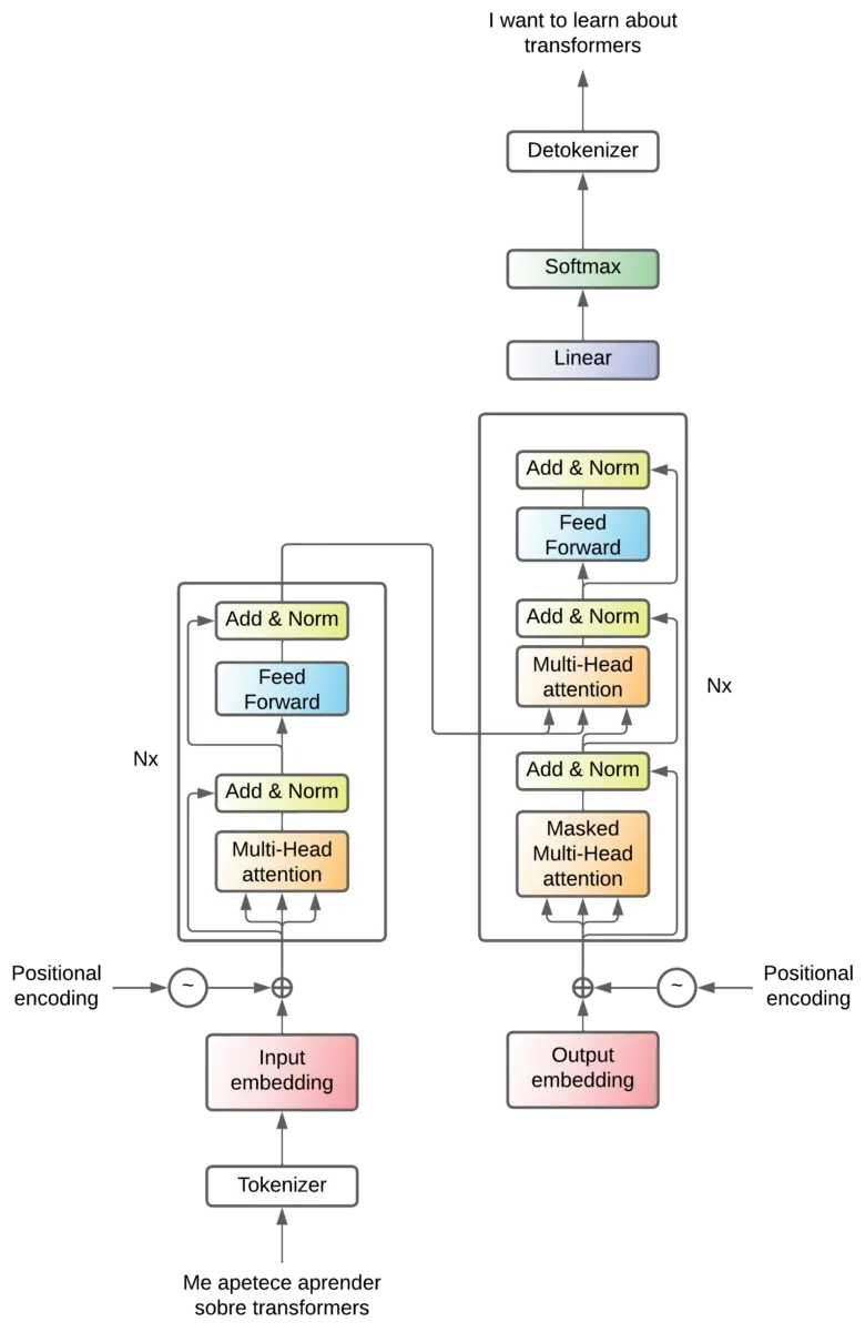
These are layers that are added after each attention layer and each feed forward layer. This layer aggregates the output and input of a layer. This is called residual connections and has the following advantages

• During training:

  • They reduce the gradient fading problem: When a neural network is very large, in the training process, the gradients become smaller and smaller as you go deeper into the layers. This results in the deeper layers not being able to update their weights well. Residual connections allow gradients to pass directly through the layers, which helps keep them large enough so that the model can continue to learn, even in the deepest layers.

  • Enable training of deeper networks: By helping to mitigate the problem of gradient fading, residual connections also facilitate the training of deeper networks, which can lead to better performance.

• During inference:

  • They allow the transmission of information between different layers: As the residual connections allow the output of each layer to become the sum of the input and output of the layer, information from the deeper layers is transmitted to the higher level layers. This can be beneficial in many tasks, especially where low-level and high-level information can be useful.

  • Improve model robustness: Since residual connections allow layers to learn better in deeper layers, models with residual connections can be more robust to perturbations in the input data.

  • They allow the recovery of lost information: If some information is lost during the transformation in some layer, the residual connections can allow this information to be recovered in the subsequent layers.

This layer is called Add & Norm, we have seen the Add, let's see the Norm. The normalization is added so that adding the input and output does not trigger the values.

We have already seen all the high-level layers of the transformer.

so we can now look at the most important part of the paper and the one that gives it its name, the attention mechanisms.

Mechanisms of attention

Multi-head attention

Before looking at the actual mechanism of attention we have to look at the multi-head attention.

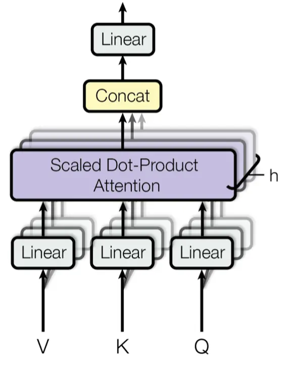
When we have explained the high-level layers, we have seen that in the attention layers there are 3 arrows, these are Q, K and V. They are matrices that correspond to the token information, in the case of the encoder attention mechanism, they correspond to the tokens of the original language sentence, and in the case of the decoder attention layer, they correspond to the tokens of the sentence that has been translated so far and of the encoder output.

Actually now we don't care about the origin of the tokens, just keep in mind that they correspond to tokens. As we have explained the tokens are converted to embeddings, so Q, K and V are matrices of size ($n_{tokens}$ x $d_{model}$). Normally the embedding dimension ($d_{model}$) is usually a large number, such as 512, 1024, 2048, etc (it does not have to be a power of 2, these are just examples).

We have explained that embeddings are vector representations of tokens. That is, tokens are converted to vector spaces in which words with similar semantic meaning are close together.

Therefore, of all these dimensions, some may be related to morphological characteristics, others to syntactic characteristics, others to semantic characteristics, and so on. Therefore, it makes sense to calculate the attention mechanisms between dimensions of embeddings with similar characteristics.

Recall that attentional mechanisms look for similarity between words, so it makes sense that similarity is sought between similar features.

Therefore, before calculating the attention mechanisms, the embedding dimensions are separated into groups of similar characteristics, and the attention mechanisms between these groups are calculated.

And how is this separation done? It would be necessary to look for similar dimensions, but to do this in a space of 512, 1024, 2048, etc. dimensions is very complicated. Besides, it is not possible to know which characteristics are similar and in each case the characteristics that are considered similar will change.

Linear projections are used to separate the dimensions into groups. That is, the embeddings are passed through linear layers that separate them into groups of similar characteristics. In this way, during the training of the transformer, the weights of the linear layers will change until reaching a point where the grouping is done in an optimal way.

Now we may have the doubt of how many groups to divide into. In the original paper they are divided into 8 groups, but there is no reason for them to be 8, I guess they tried several values and this was the one that worked best for them.

Once the embeddings have been divided into similar groups and the attention in the different groups has been calculated, the results are concatenated. This is logical, suppose we have an ebedding of 512 dimensions, and we divide it into 8 groups of 64 dimensions, if we calculate the attention in each of the groups, we will have 8 matrices of attention 64 dimensions, if we concatenate them we will have a matrix of attention 512 dimensions, which is the same dimension that we had at the beginning.

But concatenation makes all the features belong together. The first 64 dimensions correspond to one feature, the next 64 to another, and so on. So to mix them back together again, a linear layer is passed again that mixes all the features. And that blending is learned during training.

Scale dot product attention

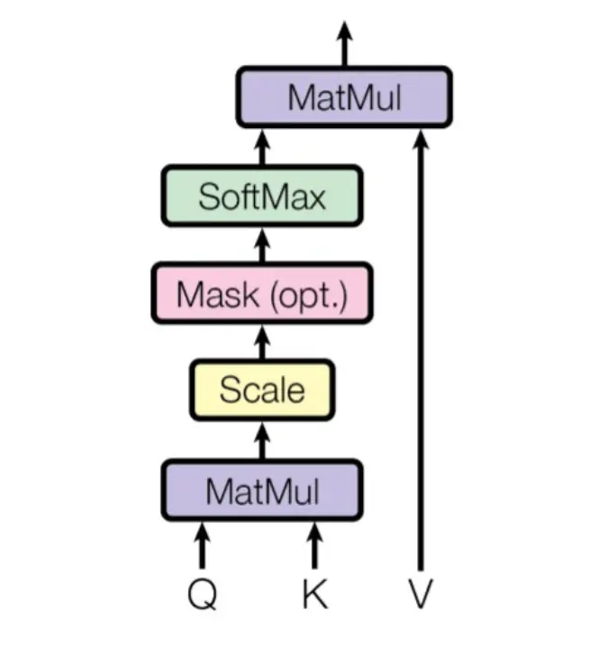
We come to the most important part of the transformer, the attention mechanism, the scaled dot product attention.

As we have seen, in the Transformer architecture there are three attention mechanisms

The encoder, the decoder and the encoder-decoder. So let's explain them separately, because although they are almost the same, they have some small differences.

Endocer scale dot product attention

Let's take another look at the block diagram and the formula

First let's understand why there were three arrows entering the attention layers. If we look at the architecture of the transformer, the encoder input is split into three and enters the attention layer

So K, Q and V are the result of embedding and positional encoding. The same array is put into the attention layer three times. We have to remember that that matrix consisted of a list with all tokens ($n_{tokens}$), and each token was converted into a vector of embeddings of dimension $d_{model}$, so the dimension of the matrix will be ($n_{tokens}$ x $d_{model}$).

The meaning of K, Q and V comes from the key, query and value databases. The attention mechanism is passed the Q and K arrays, i.e., the question and the key, and the output is the V array, i.e., the answer.

Let's look at each block separately and we will understand this better.

Matmul

This block corresponds to the matrix multiplication of the matrices Q and K. But in order to perform this operation it must be done with the transposed matrix of K. Since the two matrices have dimension ($n_{tokens}$ x $d_{model}$), in order to multiply them, the matrix K has to be transposed.

So we will have a multiplication of a matrix of dimension ($n_{tokens}$$ x $d_{model}$$) by another matrix of dimension ($d_{model}$$ x $n_{tokens}$), so the result will be a matrix of dimension ($n_{tokens}$$ x $n_{tokens}$).

As we can see, the result is a matrix where the diagonal is the multiplication of the embedding of each token by itself, and the rest of the positions are the multiplications between the embeddings of each token.

Now let's see why this multiplication is done. In the previous post Measure of similarity between embeddings we saw that one way to obtain the similarity between two embedding vectors is by calculating the cosine

In the previous figure it can be seen that the multiplication between the matrices Q and K corresponds to the multiplication of the embeddings of each token. The multiplication between two vectors is performed in the following way

$.

That is, we have the multiplication of the norms by their cosine. If the vectors were unitary, that is, their norms were 1, the multiplication of two vectors would be equal to the cosine between both vectors, which is one of the measures of similarity between vectors.

So as in each position of the resulting matrix we have the multiplication between the embedding vectors of each token, in reality, each position of the matrix will represent the similarity between each token.

Recall what embeddings were, embeddings were vector representations of tokens in a vector space, where tokens with semantic similarity are close together.

So with this multiplication we have obtained a similarity matrix between the tokens of the phrase

The elements of the diagonal have maximum similarity (green), those of the corners have minimum similarity (red), and the rest of the elements have intermediate similarity.

Scale

Let's look again at the scaled dot product attention diagram and its formula

We had said that if by multiplying Q by K we performed the multiplication between the embedding vectors, and that if those vectors had norm 1, the result would be the similarity between the vectors. But since the vectors do not have norm 1, the result can have very high values, so it is normalized by dividing by the square root of the dimension of the embedding vectors.

Mask (opt)

Masking is optional and is not used in the encoder, so we will not explain it for the moment in order not to confuse the reader.

Softmax

Although we have divided by the square root of the dimension of the embedding vectors, we could do with the similarity between the embedding vectors going between the values 0 and 1, so to make sure of that, we pass through a softmax layer.

Matmul

Now that we have a similarity matrix between the embedding vectors, let's multiply it by the V matrix, which represents the embeddings of the tokens.

By multiplying, we obtain

We obtain a matrix with a mixture of embeddings with their similarity. In each row we obtain a mixture of the embeddings, where each element of the embedding is weighted according to the similarity of the token of that row with the rest of the tokens.

In addition we have again a matrix of size ($n_{tokens}$ x $d_{model}$), which is the same dimension we had at the beginning.

Summary

In summary, we can say that the scaled dot product attention is a mechanism that calculates the similarity between the tokens of a sentence, and from that similarity, calculates an output matrix that corresponds to a mixture of embeddings weighted according to the similarity of the tokens.

Decoder masked scale dot product attention

We look again at the architecture of the transformer

As we can see in this case the scaled dot product attention has the word masked. First we will explain why this masking is necessary, and then we will see how it is done.

Why mask

As we have said, the transformer was initially conceived as a translator, but in general, it is an architecture to which you put a sequence and you get another sequence. But at the time of training you have to give it the input sequence and the output sequence, and from there the transformer learns to translate.

On the other hand, we have said that the transformer generates a new token each time. That is, it is given the input sequence in the encoder and a special start sequence token in the decoder, and from there it generates the first token of the output sequence.

Then the input sequence is put back into the encoder and the token previously generated in the decoder, and from there it generates the second token of the output sequence.

Then the input sequence is put back into the encoder and the two tokens previously generated in the decoder, and from there it generates the third token of the output sequence.

And so on until it generates a special end-of-sequence token.

But in training, as the input and output sequences are put into it all at once, we need to mask the tokens that it has not yet generated so that it cannot see them.

Mask

Let's take another look at the block diagram and the formula

The masking is done after the Scale and before the Softmax. As we need to mask the "future" tokens what can be done is to multiply the resulting Scale matrix by an array that has 0 in the positions we want to mask and 1 in the ones we don`t.

By doing this we get the same matrix as before but with masked positions

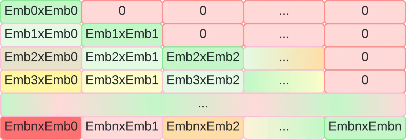
Now the result of the Scaled dot product attention is a matrix with the embeddings of the tokens weighted according to the similarity of the tokens, but with the tokens that should not be masked.

Encoder-decoder scale dot product attention

We look again at the architecture of the transformer

We see now that the attention mechanism receives twice the encoder output and once the masked attention of the decoder. So K and V are the encoder output, and Q is the decoder output.

Therefore in this attention block, first the similarity between the decoder sentence and the encoder sentence is calculated, i.e. the similarity between the sentence that has been translated so far and the original sentence is calculated.

This similarity is then multiplied by the encoder sentence, i.e. a mixture of the embeddings of the original sentence weighted according to the similarity of the translated sentence so far is obtained.

Summary

We have walked through the transformer from the highest level to the lowest level, so you may already have an understanding of how it works.